Written by: Raul Rogerio Pimentel Ribeiro
Water Pump and Pipeline Sizing

Although it is a basic and well-stablished device, a water pump performs an important role in the water supply. There are different designs of the water pumps. The most common ones are the centrifugal (dynamic) and positive displacement types. The centrifugal pump is widely used to multiple ends such as pumping water. The principal of using centrifugal pumps is transferring energy to a fluid (originally stationary) by a centrifugal force generated by an impeller with multiple blades (Palgrave, R., 2003). The principle is illustrated by figure 1.

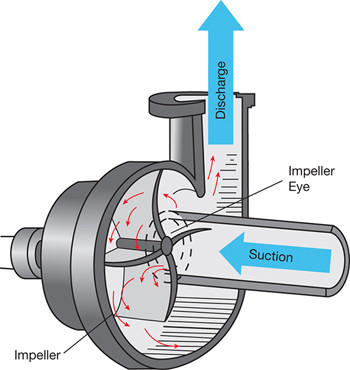
Figure 1: Principle of the function of the centrifugal pump (OEM Panels, 2018)

As it is shown above, the incoming fluid enters at the impeller eye, the impeller adds velocity energy into the liquid by the rotation of the impellers and pushes it to the direction of the discharge gate. This configuration carries many advantages that make this option the most feasible to the application proposed in this project. The centrifugal water pump configuration is suitable to high flow rates, relative higher speeds, the cost of installation and maintenance is lower due to the wide use of the technology and its simplicity (Shiels, S., 2004).

The sizing of the water pump depends on the flow rate of liquid, specific gravity of the liquid, the vertical dislocated distance of the liquid, and the efficiency of the machine. The force of friction to move the water into the pipelines. This value depends on the material, and pipe dimensions. It should be considered and calculated as the unit length which represents the ‘added distance’ to pump the water (Shiels, S., 2004). The generic formula to calculate the power required is given below:

W = (d x Q x ρ) / 3960 x η

Where

W = power (HP)
d = total distance (ft)
Q = flow rate (gallons/min)
ρ = specific gravidity
η = efficiency

Complementary, the definition of pipeline sizing is required. In order to size the pipeline, the flow rate equation is used as described below:

Q = v x ø

Where

Q = flow rate (m3/s)
v = velocity (m/s)
ø = cross-section area (m2)

The combination of these two equations generates the simplified dimension of the water pump system.

Desalination System

Technology principle: Reverse Osmosis

As the name suggests, reverse osmosis follows the principle of osmosis, however, it is applied for a job in order to generate the reverse effect. Before approaching the reverse osmosis, the concept of osmosis is a natural phenomenon that consists of the movement of water between environments with different concentrations of solutes separated by a semipermeable membrane. This principle is an important physicochemical process in the survival of human cells. The movement of water is spontaneously from the hypotonic environment which has less solute concentration to a hypertonic environment that has more solute concentration. This exchange ceases when the system matches the equilibrium which means null osmotic pressure.

Based on this concept, the reverse osmosis is a separation process that induces the solution of a region of high solute concentration through a membrane to a region of low solute concentration, through the application of an external pressure that exceeds the osmotic pressure as shown in figure 2.

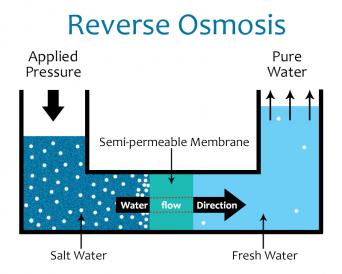
Figure 2: Reverse osmosis schematic (Green living, 2019)

As illustrated above, a semi-permeable membrane is responsible to retain the solute and allow the water flow.

Plant

The desalination system is composed of a pump to extract seawater and feed the RO plant. There is a pre-treatment which is a two-stage filter in order to avoid particles that may be in the seawater. After this stage, the water is pressurised around 50-60 bar and directed to the first stage of RO membrane modules which are named as pressure vessels. The first stage is capable to desalinate around 48-50% of the water flow (Sadhwani, J. J., & Ilurdoz, M. S. D., 2019). After that, the brine (saline concentrate liquid) is piped to the second stage of membranes. The second stage is applied in order to improve the quantity of water recovery in the process and, hence, increase the efficiency of the system (Zarzo, D., & Prats, D., 2018). The overall water recovery is around 70-75% (Zarzo, D., & Prats, D., 2018). After the second stage, the brine will retain circa 99% of the incoming salt quantity. The schematic of this process is illustrated in figure 3.

Figure 3: Desalination system

Beyond the high level of saline concentration, the brine also retains most of the pressure of the system. This pressure may be reinputted within the system instead of disposing of it immediately. The process of recovering the remained energy is called the Energy Recovery System (ERS) (Urrea, S. A., et al., 2019).

RO Membrane Module

The reverse osmosis membrane module is responsible to retain the solute of fluid and allow the water flows in order to separate it. The module applied in pressure vessels is the spiral wound membrane element whose level of purification depends on membrane type. RO membrane has the highest level of purification. Its constructions is a junction of different elements such as feed channel spacer (allows incoming flow), the membrane (filtrate the water flow), and a permeant collection material (conduct the filtrated water). Those elements are isolated from each other and multiplied inside the module. In the centre of the module, a perforated tube is designed in order to conduct the freshwater (final product). Figure 4 shows an illustration of the RO membrane module.

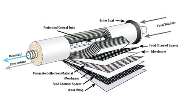
Figure 4: RO Membrane Module (Safe Technologies & Services – Reverse Osmosis Systems, 2019)

The pressure vessel is a pipe in which it contains multiple RO membrane modules (around 5 to 7) with the central tubes connected in series. The extremities of the pipe are sealed to maintain the pressure established by the pressure pump. Those pressure vessels can be connected in series with other pressure vessels in order to improve the desalination system.

Energy Recovery System (ERS)

The energy transfer using a pressure exchanger is based on using the high pressure of a fluid stream in order to power a low-pressure one. A system such as desalination ones are processes that its waste remains with a high pressure once the pressure of the fluid is barely affected when it flows into the pressure vessels. Many industrial processes operate at elevated pressures and have high-pressure waste streams. The integrated system is illustrated in figure 5.

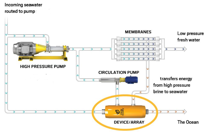
Figure 5: Energy Recovery System combined with the main desalination plant (PX Pressure Exchanger, 2020)

The high-pressure reject concentrate from the reverse osmosis plant membranes flows into the ERS, instantly, low-pressure seawater enters into the ERS and fills the rotor which is briefly exposed to the reject concentrate (brine). The energy from the hydraulic pressure is then transferred from the brine to the low-pressure incoming seawater. This pressurised seawater feeds back the system and the low-pressure reject concentrate is pushed out by the low-pressure seawater (Urrea, S. A., et al., 2019). The rotor works as a piston transferring pressure energy from brine seawater. Due to its small quantity of mobile components, the lifecycle is extended (up to 30 years) and, hence low demand for maintenance. An illustration of the principle of function is shown in Figure 6.

 

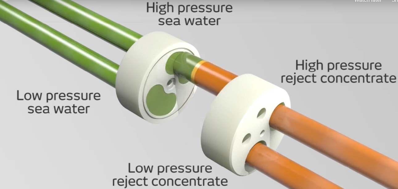
Figure 6: Energy Recovery principle of function (PX Pressure Exchanger, 2020)

The energy recovery does not only provide lower energy demand to the system but also enables smaller devices to be suitable on the desalination plant. The water pressure pump is an example. Once the recovery system injects high-pressure seawater into the main system, the main water pressure pump can be resized. The pressure recovery can pump seawater up to 25% of the system capacity (90% of the pressure rejected) (Ghaffour, N., et al., 2015). This benefit reflects into the overall cost of the system, maintenance, and system safety. On the other hand, the concentration of salt in the brine remains the same, and either lower or higher pressure, the system still has the brine to be disposed of.

Compressor System

It is observed in the specialized literature that the construction principles are divided into two groups that cover all types of existing compressors. Dynamic compressors have a rotating instrument called a rotor and their function is based on transforming energy from an external source into mechanical energy for the fluid, which in turn is moved to a blade system with the function of transforming kinetic energy into enthalpy, which is mostly translated into increased pressure. (SANTOS et al., 2006)

Volumetric or positive displacement compressors, on the other hand, act intermittently in their essence, but when a cyclical operating regime is adopted, its occurrence makes this process continuous when analyzed on a larger time scale. The performance of the volumetric compressor is based on the reduction of the volume occupied by the gas, thus increasing its pressure. Initially, a quantity of gas is admitted inside the machine’s compression chamber, which then undergoes a reduction in volume. This gas is subsequently released for storage in tanks and later consumption. These two groups are subdivided into four other groups, with characteristics that are also constructive, alternative, rotating, centrifugal, and axial. Within the rotary, there are three different construction aspects, which are the screw model, reeds, and lobes. The string of compressor types is illustrated in figure 7.

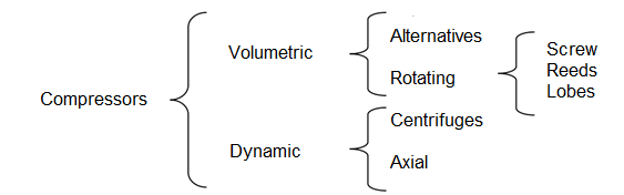
Figure 7: String of compressor types

Piston-type Volumetric Compressors

Reciprocating piston volumetric compressors have four fundamental parts: stator, rotor, pistons, and valves. The rotor has the dynamic function of this compressor by a rotating system. The pistons are located inside the cylinders and are responsible for pressurizing the air in the pressurization chamber formed by these and the cylinder walls. The valves, in turn, have a sealing function, allowing unidirectional movement of pressurized air.

When the piston is moved to increase the volume of the pressure chamber, an inlet valve opens, releasing gas into the chamber. When the piston reaches its maximum displacement over the inlet stroke, the valve closes, and the piston starts its compression stroke. This serves to compress the gas contained inside the chamber formed by the piston inside the cylinder, and when it reaches its maximum stroke, the outlet valve opens and the compressed gas is expelled to some type of closed system, under pressure for later use. , or storage. At this point, the outlet valve closes and the cycle starts over.

Among these principles, some information is relevant, such as:

• Compression occurs discreetly, within cycles (alternate movement);
• The number of pistons reflects the compressor’s pressurization capacity;
• There is symmetry between the pistons of a given compressor;

Its volumetric efficiency decreases with the increase of the reservoir pressure and its harmful space varies with the number of pistons. (SILVA, 1980). Figure 8 illustrates the piston compressor, an example to illustrate the working principle of a compressor.

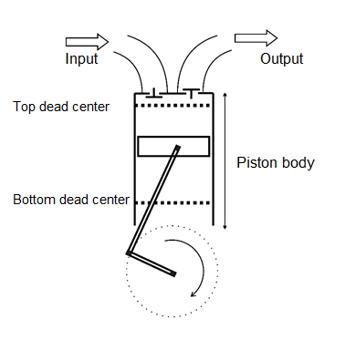
Figure 8: Principle of the function of the piston-type compressor.

The energy required to compress a gas is dependent on factors such as temperature, pressure, volume, and the configuration of the system (number of stages). Ideally, the compression process can be considered as adiabatic (constant temperature) in order to simplify the calculation workload (DOE, 2009). Due to this consideration, the theoretical power demand to compress a gas is defined by the formula:

A = (144N x P1 x V x k) / [33000 x (k-1)]

B = {[P1^(k-1/Nk)] / P2 } – 1

HP = A x B

Where

HP = power of compressor (HP)

N = number of compression stages

k = adiabatic expansion coefficient

P₁ = input pressure (psi)

P₂ = output pressure (psi)

V = Volume flow of the gas in atmospheric pressure (ft³/min)

The adiabatic expansion coefficient (specific heat ratio) is the ratio between isobaric specific heat (c_p) and isochoric specific heat (c_v) and in the case of hydrogen gas (H₂), the constant k is equal to 1.405 (Peschka, W., 1992). Although the theoretical power required has been defined. The compressor sizing should consider friction losses and heat losses. The friction and heat losses vary between 10-20% of the theoretical power required (Bracha, M., et al., 1994)(DOE, 2009). In order to achieve a fair dimension for the compression system, the maximum friction and heat losses will be considered.

Transformation System

Power Transformer

There is the demand for transforming high AC voltage into low DC voltage for matching the requirements for the use of electrolysers. Transforms are, among other applications, designed in order to transform (change) voltage and current levels in order to meet system demands (Green Energy and Technology, 2009). The basic understanding of transformers is that the power input must match with the power output in an ideal transformation which is described below.

e1/e2 = i1/i2 = N1/N2

Where e1 and e2 are respectively the input and output voltage, the i1 and i2 are the input and output current, and N1 and N2 are the primary and secondary windings as shown in figure 9.

Figure 9: Transformer operation

The AC current which flows into the primary coil generates a magnetic flux Φ that links the primary coil with the second one and generates an electric voltage (e2). This voltage is directly proportional to the relation between primary and secondary windings. The current follows a reversed proportion which allows the power to remain its initial value (Green Energy and Technology, 2009).

The transformers are real devices such as any other, thus it also performs losses during the transformation process. A non-ideal transformer includes losses of magnetization (Xm) which is based on the required current of magnetization. Also, it performs iron losses( Rfe) which comes from Eddy losses and hysteresis losses. Those two previous points represent the excitation loss of the system (Wildi, T., n.d.). The windings of the transformer also deploy some losses from the resistance of the material utilised which is so-called as copper losses (Rs). This loss is found on both sides of the transformer. Finally, the leakage of the magnetic flux (Xs) is also accounted as loss once not all the magnetic flux travels from the primary to the secondary terminal of the transformer and it is also considered on both terminals (Wildi, T., n.d.). These losses are considered to provide the schematic of a non-ideal transformer as figure 10 shows.

Figure 10: Non-ideal transform with all transformation losses

Based on these schematic, the efficiency () of the transformer may be obtained from ration between the product of output voltage (V2) and current (I2), and the input voltage (V1) and current (I1). These input values can also be identified by adding the power of losses to the power output as shown below.

The efficiency of a power transformer is usually around 95-98% which does not affect much the cost of energy production. The losses are more related to heat that is easily found on transmission (Wildi, T., n.d.).

After transforming the power into a determined voltage level, the necessity of converting this AC voltage into DC voltage becomes essential.

AC/DC Converters (Rectifier)

The configuration to convert AC to DC is called a rectifier and there are a number of possible configurations in order to produce it. The most used configuration is the full-wave rectifier which may be explained as a configuration that carries out full-wave rectification (Cooley, G. C., 2013). The concept consists in maintaining the current flowing in the same direction (Gao, D. W., 2015). In an ideal circuit, the value of DC voltage on behalf of a single-phase full-wave rectifier corresponds to the RMS value of AC voltage as shown below (Martinez-Velasco, J. A., 2015).

Vdc = Vrms = Vac/2^(1/2)

The single-phase full-wave rectifier can be controlled or uncontrolled. The uncontrolled rectifier is defined by the use of diodes that when it is directly polarised, the diode allows current flow. On the other hand, when it is reversed polarised, the diode cuts off the current flow (Martinez-Velasco, J. A., 2015). A sample configuration is shown below in figure 11.

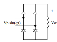
Figure 11: Schematic of single-phase full-wave rectifier

In this particular case, the resistive load does not affect the format or position of the wave format once the power factor of a resistive load is equal to 1. The wave format is shown in figure 12.

 

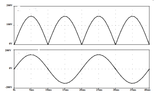
Figure 12: Input voltage shape (lower) and rectified output voltage

As it can be observed, there is no negative voltage after rectifying the voltage signal. However, this fluctuation in the DC voltage is not desired (Gao, D. W., 2015). In order to develop a better output shape, the implementation of the filter is necessary in order to balance the voltage output and levels. This levelised voltage output can be achieved by allocating a capacitor in parallel with the resistive load (Gao, D. W., 2015) as it is shown in figure 13.

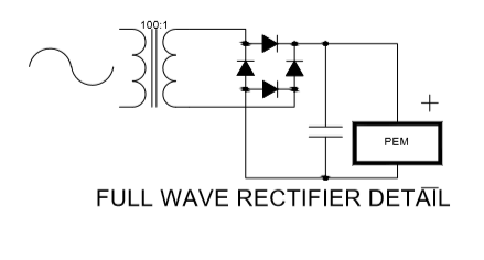
Figure 13: Full-wave rectifier detail

The capacitive filter works as a current source that stores electrical energy and discharges to the load during the reduction of the instantaneous voltage output value. Thus, a new wave is reshaped as displayed in figure 14.

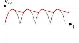
Figure 14: Voltage output after implementation of a capacitive filter

The difference between the peak and the lowest voltage value produced by the capacitor discharge is named as ripple (Gao, D. W., 2015). The ripple can be obtained by the equation below.

Vripple = Vpeak / (f x C x R)

Where the denominator is the product between frequency f, capacitance C, and the load R. Observe that the capacitance (size of the capacitor) may generate a lower ripple which can contribute to higher signal stability (Martinez-Velasco, J. A., 2015). The decrease of the ripple means a DC output equal to the peak value of the AC input without considering losses in diode polarisation.

The same concept may be applied for a three-phase system which is likely to be the case of wind energy production. Respecting the same concept, the circuit of a three-phase rectifier is shown in figure 15.

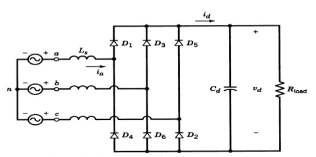
Figure 15: Uncontrolled three-phase full-bridge Rectifier configuration

It is required six electronic devices in order to actuate as a rectifier. The case above shows a circuit with diodes. Thus, the system rectification is uncontrolled (Gao, D. W., 2015). In order to illustrate the voltage variance in the load (voltage waveform), figure 16 is displayed below.

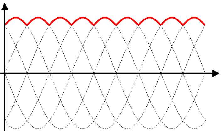
Figure 16: Three-phase rectifier voltage waveform in the load

As it is noticed, the fluctuation of the DC signal is sensibly lower compared to the single-phase rectifier waveform. The application of the capacitor filter performs an even lower variation which may generate a satisfactory flat waveform. The necessity of filter and controlled rectifiers are related to the profile of output desired and application of the designed system (Patin, N., 2015).

REFERENCES

BOTT, R. Compressores Portal Indústria. 2018.

Bracha M., et al., “Large-Scale Hydrogen Liquefaction in Germany” International Journal of Hydrogen Energy 19 (Jan 1994) pp. 53-59.

Buckley, C., Simpson, Kerr, & Schutte. (1987). The treatment and disposal of waste brine solutions. Desalination, 67(C), 431-438.
Cooley, G. C. (2013). Electrolysis for Efficient Offshore Wind Energy Storage. SoapBox, 69.

Felgenhauer, T. Hamacher, State-of-the-art of commercial electrolyzers and onsite hydrogen generation for logistic vehicles in South Carolina, Int. J. Hydrogen Energy 40 (2015) 2084–2090.

Gao, D. W. (2015). Energy storage for sustainable microgrid. Amsterdam: Academic Press. Elsevier.

Gardiner, M. (2009). Energy requirements for hydrogen gas compression and liquefaction as related to vehicle storage needs. DOE Hydrogen and Fuel Cells

Program Record, 9013. Retrieved from https://www.hydrogen.energy.gov/pdfs/9013_energy_requirements_for_hydrogen_gas_compression.pdf

Ghaffour, N., Bundschuh, J., Mahmoudi, H., & Goosen, M. F. (2015). Renewable energy-driven desalination technologies: A comprehensive review on challenges and potential applications of integrated systems. Desalination, 356, 94–114. doi: 10.1016/j.desal.2014.10.024

Hart, O. O., Groves, G. R., Buckley, C. A., & Southworth, B. (1983). A guide for the planning, design and implementation of wastewater treatment plants in the textile industry. Part one: Closed loop treatment/Recycle system for textile sizing/desizing effluents. Pretoria.

Hydrogen Generation from Wind Power. (2009) In: Stability Augmentation of a Grid-connected Wind Farm. Green Energy and Technology. Springer, London

Juan A. Martinez-Velasco, “Dynamic Average Modelling of Rectifier Loads and AC-DC Converters for Power System Applications,” in Transient Analysis of Power Systems: Solution Techniques, Tools and Applications , , IEEE, 2015, pp.360-397

Mabrook, B. (1994). Environmental impact of waste brine disposal of desalination plants, Red Sea, Egypt. Desalination, 97(1-3), 453-465.

Palgrave, R. (2003). Centrifugal pump basics. Troubleshooting Centrifugal Pumps and Their Systems. doi: 10.1016/b978-185617391-9/50018-6

Patin, N. (2015). AC/DC Converters. Power Electronics Applied to Industrial Systems and Transports, Volume 2, 101–159. doi: 10.1016/b978-1-78548-001-0.50003-4

Peschka, W. (1992). “Liquid Hydrogen.” Springer-Verlag, New York.

PX® Pressure Exchanger®. (2019). Retrieved February 9, 2020, from http://www.energyrecovery.com/water/px-prime/

Sadhwani, J. J., & Ilurdoz, M. S. D. (2019). Primary energy consumption in desalination: The case of Gran Canaria. Desalination, 452, 219–229. doi: 10.1016/j.desal.2018.11.004

Safe Technologies & Services – Reverse Osmosis Systems. (2019). Retrieved February 9, 2020, from https://sosafetechnologies.com/ro_systems

SANTOS, A. H. M. et al. Conservação de Energia: Eficiência Energética de Equipamentos e Instalações. [s.l: s.n.].

Shiels, S. (2004). Centrifugal pump specification and selection — A systems approach. Stan Shiels on Centrifugal Pumps, 1–20. doi: 10.1016/b978-185617445-9/50001-1

SILVA, R. B. Compressores, Bombas de Vácuo e Ar Comprimido. 2. ed. São Paulo: Grêmio Politécnico, 1980.

Urrea, S. A., Reyes, F. D., Suárez, B. P., & Juan A. De La Fuente Bencomo. (2019). Technical review, evaluation and efficiency of energy recovery devices installed in the Canary Islands desalination plants. Desalination, 450, 54–63. doi: 10.1016/j.desal.2018.07.013

VFD Variable Frequency Drive and Centrifugal Pump • OEM Panels. (2018). Retrieved February 9, 2020, from http://www.oempanels.com/vfd-variable-frequency-drive-and-centrifugal-pump

WILDI, T. (n.d.). Electrical machines, drives, and power systems. Pearson.

Zarzo, D., & Prats, D. (2018). Desalination and energy consumption. What can we expect in the near future? Desalination, 427, 1–9. doi: 10.1016/j.desal.2017.10.046