

| Tidal Cycle Analysis |  |
Impact of springs and neaps Impact of frequency variation Conclusions References
Impact of springs and neaps (14 day analysis)
Tidal height, and subsequently tidal speed varies greatly from springs (new/full moon) to neaps(1st and last lunar quarters) - please refer to the Tidal Principles section for more information on the nature of springs and neaps.
The main aim of carrying out a 14 day analysis was to gain an understanding of the magnitude of this variation and it's impact on the power output.
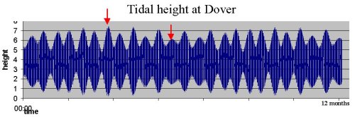
This was achieved by effectively combining the graphs of "tidal height at Dover for a 14 day period"(assuming that all sites vary their tidal height in accordance with Dover)......
....with our "sinusoidal model for power output" at a specific site.
The above model uses a value for the maximum tidal speed (based upon average spring values) to produce a sinusoidal representation of the energy output.
We needed to model how the the maximum tidal speeds in each cycle (the amplitude of the model) would vary over time, and observe how this variation would affect our graph of the energy output.
The actual data value for tidal speed we held for our given site was a spring average. Accordingly, a 14 day period for Dover with a spring tidal height value matching the average spring height value was chosen - so that that the two graphs roughly corresponded to the same periods.
NOTE - previous studies carrying out similar analyses omitted to take into account the fact that they were using the spring average, and combined the graphs on the basis that they were using the absolute peak value for the year.
The model using the average spring value for speed was shifted in time so that it alligned with the average spring value for tidal height at Dover.
In order to vary the model for our chosen location by the correct amount from one day to the next, ratios were calculated for the variation in tidal height at Dover for each day. These were based on a datum of the maximum peak for the year:
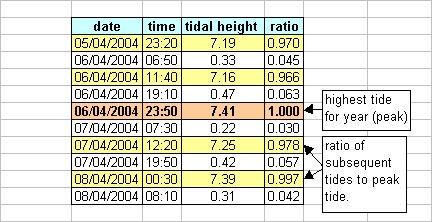
Assuming a linear relationship of variation of tidal height and variation of tidal speed, values for peak speed for each previous and subsequent tidal speed cycle for our site were then calculated using the ratio for tidal height variation, and used to extrapolate the wave form. The blue shows the potential power out, and the pink the actual power out due to the turbine specification.
The result shows a large variation in the power output throughout the cycle. However, this particular site has very high speeds, so this variation does not affect the available power output of the chosen turbine, which is low in comparison. If the speeds at the site were much lower, then the following result would be obtained:
It can be observed that the rated speed is not always reached at this site due to this 14 day variation (the graph shows a curved peak at some points rather than reaching a plateau). As such, it was decided from this analysis that we should evaluate each of our chosen scenarios on the basis of spring peak and neap tidal speed ranges (shown for Dover below). This can be viewed in more detail in the supply strategy section.
back to top
Impact of variations in time for one cycle (12.4 hour variation)
The length of the tidal cycle can vary from one cycle to the next. The purpose of this analysis was to determine the implications of this variation on the phasing of our sites, and calculate any resultant errors.
The illustration below shows the variation in length of the tidal cycle at the reference port of Oban (relatively close to many of our sites).
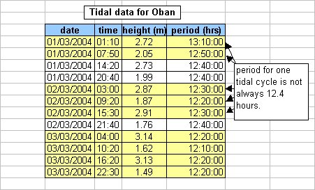
The length of the cycle appears to vary approximately in accordance with the tidal height, as shown below:
When the tidal range is largest (i.e. springs), the water moves more quickly, and so the cycle time is smallest.
When the tidal range is at a minimum (i.e. neaps), the water has less force behind it and moves more slowly, so the cycle time is longest.
A sensitivity analysis wasundertaken to determine the impact of this variation. The first stage used modelled data for a real site, but varied the time of the tidal cycle to the minimum and maximum values (12hrs and 13.4hrs respectively) and plotted these against the standard model. The resultant graph (below) showed that the impact of this variation on one cycle was small, but as time went on, if this extreme variation continued the cycle would move substantially from its expected position.
However, through implementing this analysis it was realised that:
- 8.5% of the time in the chosen case study, the value matches 12.4
- A variation of the maximum or minimum value twice in a row (across two cycles) would be highly unlikely,
- The variation will correct itself over time as we move from spring to neaps and back,
- An assumption that all sites vary in length of tidal cycle by the same amount it valid, and therefore the impact of this variation on the phasing of sites is negligible - if one site moves, all move.
To test the observation that the variation corrects itself over time, an error to account for the positive and negative variation from the 12.4 hour cycle was calculated. This error proved to be relatively small - only plus or minus 1%.
back to top
Conclusions
The variation in spring and neaps speeds is an important consideration when assessing the potential baseload that can be obtained from a site - if we are trying to obtain a flat output from our sites, we may be restricted by the output at springs (depending upon site speeds).
The variation in frequency, which we initially thought to be a major issue, has a negligible impact on site phasing (the timing of the sine wave at each site, and how these relate to one another), as based on the best information we currently have access to, this will impact all sites in the same way. This will however be required in order to provide an accurate prediction of storage requirements or peaks in the supply if a pure baseload is not obtained.
back to top
References
- Neptune Navigation, Neptune Tides Demo Package, Reading, Berkshire.
http://www.neptune-navigation.com.
back to top