Energy Analysis - Methodology

Home

project outline

Background

why marine currents?
policy
economics
environment
planning
grid connection

Technology

concepts
decisions
considerations
performance
storage options

Resource basics

tidal principles
methodology
tidal variations
map of resource

Site Analysis

transmission network
areas avoided
seabed morphology
user conflicts
navigational risk
selected areas
results

Energy Analysis

theory
methodology
power calculations

Supply Strategy

introduction
site selection
phasing
use of storage
Min storage strategy
Max storage strategy

Economics

electricity cost
socio-economics
market factors

Environment

emissions analysis
environmental impact

Conclusions

summary
conclusions
future work

Team work

team members
logbook
acknowledgements

Glossary

definitions

References

links
publications

Methodology

Parametric Model Power Profiles Error Estimation

This section gives an overview of the method employed in the generation of the power profiles for the sites as well as assumptions used and the possible errors. The turbine parametric model used has also been included.

Parametric Model

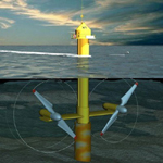
The 1 MW design described in the Commercial Prospects of Tidal Stream document prepared by Binnie Black and Veatch in association with IT Power was adopted for this study. The concept is a twin rotor (2 x 500 kW) axial flow turbine mounted on a monopile founded in the seabed as shown below.

Key characteristics of model
Characteristic	Units	Value
Rated power	kW	1000 (2 x 500)
Rated mechanical power	kW	1120
Rated speed	m/s	2.4
Cut-in speed	m/s	0.7
Rotor rated speed	rpm	14.4
Rotor Diameter	m	15.85
Power Coefficient	-	0.4
Gearbox transmission efficiency	-	0.95
Generator efficiency	-	0.94
Output voltage	V	690

Key features:

Variable-pitch mechanism allowing rotor blades to be adjusted through at least 1800so they can operate during both flood and ebb flows.
The twin rotors are contra-rotating to minimise resultant forces on the support structure.

The speed variation with time was assumed to be sinusoidal completing a cycle every 12 hr 25 min. The maximum (reference) speed was taken as the mean of the mean neap and mean spring tides for both flood and ebb flow. The speeds were generated at one minute intervals. The chart tidal speeds were then compared to the sinusoidal speeds to estimate the level of accuracy.
Armed with the sinusoidal speed variation and a choice of turbine parameters the available power for each speed was calculated. The actual power was then found by multiplying the available power by the power coefficient taking into account the rated speed of the turbine. This was then converted to electrical power output by multiplying by the gearbox transmission efficiency as well as the generator efficiency.
The next step was the generation of power profiles (power output against time) for the various locations for a 12 hr 25mins cycle.

A spreadsheet was generated for each location which calculates the sinusoidal speeds, the available power, mechanical power output as well as the electrical power output at one minute intervals.

back to top

Error Estimation

The two main assumptions underlying the analysis are:

Sinusoidal variation of tidal speeds
12 hr 25 min cycle repeating itself over time

Actual tidal speeds do not follow a sinusoidal variation and also do not always undergo a 12 hr 25 min cycle. The level of deviation from the actual tide behaviour is therefore crucial to the accuracy of the results. The purpose of this section is therefore to investigate the effects of these simplifying assumptions. The hourly tidal speeds from charts were superimposed with the sinusoidal speed variation and the deviation calculated by comparing the areas under the two graphs using the trapezium rule. It is worth noting that tidal data at one hour interval is not very indicative of true speed variation. A shorter time interval would have resulted in a better error estimation as the shape of the curve between two hourly points is approximate.

back to top