

| Methodology |  |
Introduction Initial study Target Speed and Depth Tidal stream data capture
Tidal times Data validation References
Introduction
The aim of this stage was to complete a detailed study of the Tidal Stream (or Marine Current) resource in Scotland and identify best sites of high tidal stream speeds at the correct depths to install Marine Current Turbine schemes and convert this marine energy into electricity.
The maximum speed of the tidal stream either side of HW - the ebb and flood - during both Spring and Neap tides were captured for several locations around Scotland, as shown in the chart below for Kyle of Rhea.
Figure: Kyle of Rhea Tidal Stream speeds plotted against time
The mean maximum speed was then calculated. The times of high-water (HW) and low-water (LW) at which the minimum speeds occur were also captured for each site. These values were then used to calculate the potential power available for each site in the Energy Analysis stage of the project.
back to top
Target speed and depth
The Marine Current Turbine the selected technology in this project to exploit the resource requires average speeds of around 2 meters per second or greater. The depth of the area of water was also very important when identifying potential sites. It was assumed that the first generation of commercially available Marine Current Turbines, using the monopile support structure, could be installed in depths of 20-50 metres. For depths between 50-80 metres, it was assumed that the second generation of MCTs, using an alternative support technology would be exploit the resource. These assumptions are consistent with Marine Current Turbines ltd.
back to top
Initial study of tidal stream resource
An initial study of the Marine Current resource in Scotland was carried out. Using previous studies of the UK resource, key sites of high-current velocity on the Scottish coastline were identified. An initial list of marine and coastal sites, which experienced the required speeds, was produced. Areas identified include Galloway, the West coast, the Pentland Firth, Orkney and Shetland.
back to top
Tidal stream data capture
Using the initial locations as a starting point, a more detailed study of the tidal currents was completed to capture the additional data on the tidal speeds that would be required to estimate the potential power and energy that might be captured from each site.
- 14-Day cycle Spring and Neap speeds
- 12.4 Hour cycle speeds (and the Sinusoidal pattern)
- Ebb and Flood speeds
- Data Source - Tidal Stream Atlases and Admiralty Chart Tidal Diamonds
Tidal speeds vary from day-to-day as the earth rotates through the 14-Day cycle from spring to neaps tides (the times with maximum and minimum tidal height ranges respectively). The tidal speeds during Spring tides are much faster than the speeds during neap tides because the amount of water that is displaced as the tides flows in and out is much less during neaps. Using only spring speeds as used in previous studies would prevent the tidal stream behaviour being accurately modelled over an annual period because the lesser tidal stream speeds incurred during neap tides would not be included and the resource would be over estimated. To account for this 14-day cycle and the large variation in speeds that occur - variations of between 50-75% - the neap speeds must also be captured. A mean speed can then be calculated using the average of these speeds (see Tidal principles section for more details).
The strength of the tide also varies during the day between successive high or low waters which takes an average of 12.4 hours from HW to LW back to HW. The speed varies from its minimum speed of zero at times of slack water at HW (or LW), and increases to its maximum speed at approximately half-way between HW and LW. It can safely be assumed that tidal flows follow a sinusoidal pattern over this 12.4 hour cycle. Therefore is it important when attempting to model the tidal stream of a specific location to capture the peak speeds and the times at which they occur so the period can be calculated and the sinusoidal graph of the tidal speed against time can be plotted (see Tidal principles section for more details).
The speeds experienced either side of HW tend not to be symmetric. The speeds of the flood when the tide flows in from LW to HW tend to be greater than that of the ebb when the tide goes out from HW LW. Therefore it is also important to capture the both speeds during flood and ebb flows.
Using Tidal Stream Atlases and Admiralty Chart Tidal Diamonds, as shown in the figures below, the required tidal speeds for several exact positions of latitude and longitude around Scotland were captured in knots and converted to metres per second. An area around each point was selected, assuming the same tidal speeds for all currents within that area. The minimum and maximum depth were also recorded.
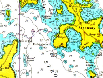
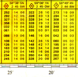
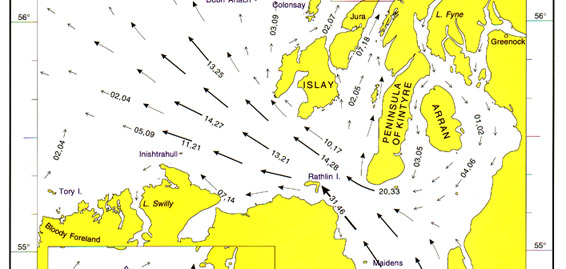
Figure: Tidal Stream Atlas, North Coast of Ireland and West Coast of Scotland
back to top
Tidal times - tidal data linking
Using Admiralty Tide Tables the times were captured for high water (HW) and low water (LW) at the UK port of Dover allowing for all of the site speeds to be plotted against time and hence link the tidal stream data for different sites together on the same graph. It was then possible to determine when the speed of a tidal stream at one site in relation to other sites. As the time of HW and LW change with respect to latitude so the times of HW and LW for the sites was distributed right across the 12.4 hour period.
The time at which each tidal speed takes place before, during and after HW Dover was collated and a graph of tidal speeds plotted against time for each location. The table and figure below shows the tidal speeds and times for the Kyle of Rhea site together with the plotted graph.
Table: Kyle of Rhea Tidal Stream speeds and times
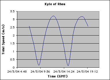
Figure: Kyle of Rhea Tidal Stream speeds plotted against time
Findings
It was observed that the maximum speeds or peaks occurred at roughly halfway between the time of HW and LW. This observation is consistent with the 'rule of twelfths' that states that half (6 twelfths) of all water that moves when the tide floods in or ebbs out travel in the 3rd and 4th hour between HW and LW. The minimum speed or troughs occurred at HW or LW or at times of slack when no tide flows. The times at which the peaks and troughs of the tidal velocity occurred for each site varied.
Hypothesis
Therefore, if the peaks of several sites are distributed across a time period of comparable length to once tidal cycle, on average of 12.4 hours, then a combined constant speed required should be maintained. Hence, if the marine energy is captured effectively a constant power source should, in theory, be attainable. Ensuring an even distribution of peak speeds forms the bases for selecting the sites effectively and should in turn allow for a constant power supply to be generated meeting a proportion of Scottish baseload.
back to top
Alternative method Tidal Data Validation
The initial method calculated when the peak speeds occurred at a site using the Tidal Stream Atlas or the Tidal Diamonds which give speeds in relation to HW of a standard UK port, which in most cases was Dover and not the times for port located close to the site. The scale of the Tidal Stream Atlases is not very detailed and accuracy of the time measurements of the Tidal Stream Tables and Chart Diamonds is not easily justified. To validate the initial times of the speeds captured, an alternative method was employed for certain sites where the maximum speed for both ebb and flood flows during Spring and Neaps was available.
Using the Tidal Stream Arrows marked on Admiralty Charts, the peak speeds for both ebb and flood flow either side of HW were capture and the mean was calculated from Spring and Neap arrow.
Assumption 1
Again assuming the tidal stream speeds can be represented for a 12.4-hour cycles using a sinusoidal equation to plot speed against time. The value of the maximum point of the peak before HW was set to the maximum Flood speed captured and maximum point of the peak after HW was set to the maximum Ebb speed captured. The minimum points of the troughs was again assumed to occur at high water and low water at times of slack when the tidal speed is 0.
Assumption 2
Assuming the Rule of Twelfths - where the fastest streams take place during the 3rd and 4th hour after slack water (HW or LW) - the maximum speeds were set exactly halfway between the minimum speeds.
Assumption 3
The times of HW and LW for local ports, located within the areas selected for each site, were taken from Admiralty Tide Times for a given 24-hour period. The times at which the minimum speed takes place were assumed equal to the HW and LW times. (However, this assumption restricted the number of sites that could be analysed using this method, as not every site was located close to a standard port.) The period of the sinusoidal curve could then be calculated and the tidal speeds were plotted against time. The new curve was then overlaid on top of the speed graph generated using the initial method to compare the techniques and validate the speeds already captured.
Findings
It was observed that this technique produced a more accurate representation of when the tidal stream peaks occurred as is used the actual times for ports located at within the sites areas selected.
The mean maximum speeds for the ebb and flood flow either side of HW and the times of HW and LW - when the minimum speeds occur - were used to calculate the potential power available for each site in the Energy Analysis stage of the project.
back to top
References
- DTI (1993), UK Tidal Stream Energy Review, ETSU.
- Commission of the European Communities, DGXII (1996b), Wave Energy Project Results:
The Exploitation of Tidal Marine Currents, Report EUR16683EN,
Commission of the European Communities.
- Binnie, Black & Veatch in association with IT Power(2001),
The commercial prospects for tidal stream power, ETSU T/06/00209/REP, HMSO.
- British Admiralty, Admiralty Tidal Stream Atlases, NP 209, NP 218
- British Admiralty, Admiralty Chart Tidal Diamonds (Positions of tabulated tidal stream data with designation)
- British Admiralty, Admiralty Tide Tables, N 201 Volume 1: United Kingdom and Ireland
back to top