

| Theory |  |
Energy conversion Trapezium rule References
Energy conversion
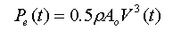
Moving water has kinetic energy similar to wind. The energy per second intercepted by a device of frontal area A0(m²) in water of density ρ, and current velocity V (m/s) is therefore given by:
The power that can be converted to a useable mechanical form is limited for a device in an open water flow to:
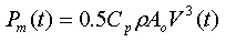
where Cp is the power coefficient. The value of Cp for a turbine exposed to the flow of and incompressible fluid is limited to a theoretical maximum value of approximately 0.593 according to Betz law. For a device the power coefficient is generally a function of the tip speed ratio (ratio between the speed of the turbine blade tip and the fluid flow speed), which is dependent on the blade form and the number of the blades.
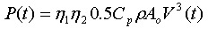
Assuming a gearbox transmission efficiency of η1 and generator efficiency of η2 then the electrical power output is given as:
Tidal currents are not constant. Generally they are a combination of quasi-steady marine currents and flows induced by the tides. Estimation of energy capture therefore becomes a fairly complex procedure. However for most sites the flows are purely tidal, making it possible to parameterise the tidal currents as series of simple sinusoids. Assuming the current velocity V(t) follows a cyclic pattern then:
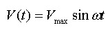
and
where:
- Vmax is the maximum current speed at the surface
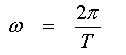
- ω is the angular velocity of the tide
- T is the period of the cycle, typically 12h 25 min or 745 minutes.
The times at which cut-in and rated power occur (relative to the start of the cycle) are indicated by T1 and T2 in below:
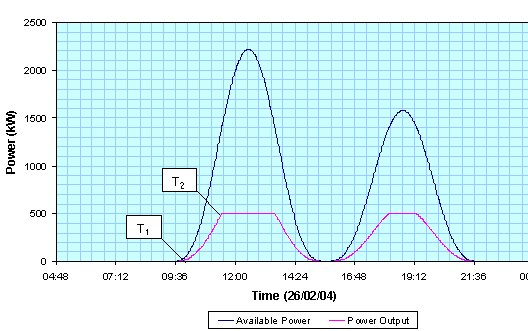
Figure 1. Power profile
A tidal current turbine will normally generate power for both flow (flood and ebb) directions, so its power characteristic (as a function of time) will be similar for each half of the cycle, however the speeds for the flood flow are generally higher than that for the ebb flow.
The energy captured is given by the area under the power curve. So the energy captured during one half of each half tidal cycle is:
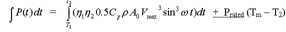
working in units of minutes for time.
Tm represents the mid-point of each half-cycle shown in Figure 1. The mean power output and capacity coefficient (same definition as for wind turbines) may then be calculated easily. Note that the turbine produces no power for a period equal to 2T1, spanning the end of one half-cycle and the beginning of the next.
back to top
Trapezium rule
The trapezium rule provides an alternative means of estimating the area under a curve. It is more useful where the curve cannot be represented by an equation. Basically it works by splitting the area under the curve into a number of trapezia. The areas of the various trapezia are then summed up giving an approximate area under the curve. Consider the curve in figure 2, the area under the curve between a and b is given by the sum of trapezia A, B, C and D of equal widths. Increasing the number of divisions increases the accuracy of the results.
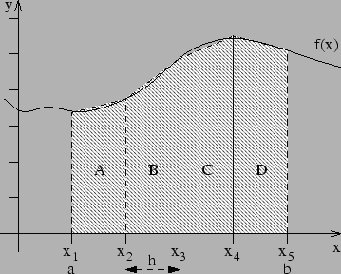
Figure 2. Curve illustrating the trapezium rule
ie:
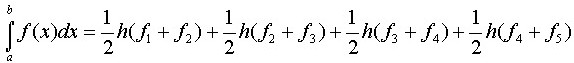
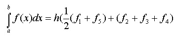
this simplifies to:
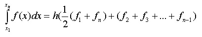
Generalising for n points we have:
back to top
References
- Bahaj, A S and Myers, L E (2003), Fundamentals applicable to the utilisation of marine
current turbines for energy production, Renewable Energy 28, 2205-2211.
- Bird, J O (1998), Mathematics for Engineers, Oxford, Butterworth Heinemann Ltd.