
 Home
Home 
| von
Karman BL Calculation |
Description of Model
In order to assess the flow, it is postulated that the section of interest, e.g. a channel, is entirely developed, fully turbulent flow. This allows us to consider it as a large boundary layer, stretching from the seafloor to the free surface, and as such calculate the velocity profile as we would a turbulent boundary layer. (6)(14)
Some nomenclature
In describing velocities and sizes of and in the boundary layer, the following notation is adopted:
|
U |
|
y |
|
u |
|
|
|
 |
|
It should be noted that when referring to velocities within the boundary layer (and by extension, all velocities in the channel), velocities in this article should considered time averaged, as in an actual turbulent flow, velocities are extremely random and it is only the tendency for net transport of the gross flow that gives rise to any coherent motion. This is acknowledged, and all flow velocities are herein assumed time averaged (as in the specification of the variables below).
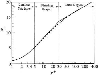
To describe these profiles physically, they may be split for convenience into three layers, characterised by their distance from the wall: an inner viscous sub-layer, an outer turbulent wake layer and an overlap layer adjoining them.
- Inner Variables:
 by
Prandtl
by
Prandtl - Outer Variables:
 by
von Karman
by
von Karman
An overlap layer exists between the inner and outer regions where both inner and outer relationships are valid.
In the outer layer, the fluid velocity increases with distance from the wall to freestream velocity, and arguments based on dimensional analysis and the derivation by Coles leads to the profile adopted in the present analysis, valid in both the overlap and outer layers (eqn 1):
 |
Eqn 1 |
 |
Eqn 2 |
| Eqn 3 | |
 |
Eqn 4, 5 |
 |
Eqn 6,7 |
-
 is
skin friction coefficient, equal to the wall shear stress non-dimensionalised
by the freestream dynamic head
is
skin friction coefficient, equal to the wall shear stress non-dimensionalised
by the freestream dynamic head -
 is
the non-dimensional velocity of the flow within the boundary
layer, equal to
is
the non-dimensional velocity of the flow within the boundary
layer, equal to 
-
 is
the non-dimensional height, in terms of BL thickness, frictional
velocity and kinematic viscosity
is
the non-dimensional height, in terms of BL thickness, frictional
velocity and kinematic viscosity  is termed the skin friction parameter, H the shape parameter,
 is Cole’s wake parameter and
  is Clauser’s equilibrium parameter which indicates a pressure
gradient dependence in the shape of the profile (in our case
it is assumed that pressure gradient is due to head difference
along the channel as opposed to an external velocity distribution).
is Clauser’s equilibrium parameter which indicates a pressure
gradient dependence in the shape of the profile (in our case
it is assumed that pressure gradient is due to head difference
along the channel as opposed to an external velocity distribution).
A full derivation and the physical meaning of these terms may be found in most fairly advanced physics of fluids textbooks, eg Frank White’s Viscous Fluid Flow (19). B and K are pure dimensionless constants, and generally accepted as being 0.4 and 5.5 respectively, although Gross (10) suggests alternative values for use in oceanic boundary layers. It is questionable whether the shallow water straits of interest may be described as being oceanic, however the constants are relatively similar (0.41 and 5.0 respectively). In all cases, they are based on experiments by Nikuradse, who would while away the hours by flowing water down drainpipes lined with sandpaper of varying gauge, arriving at his conclusion on the velocity profiles of various boundary layers.
Observations indicate that the relative sizes of the boundary layer regions is as follows:
- Inner layer: 0.1 – 1%
- Logarithmic blending region: 10 – 20%
- Outer region: 80 – 90%
And since the Coles profile is valid within the overlap and outer
regions, it is feasible that it can be applied to up to 99.9%
of the profile. As such, it is the approach adopted in this project.
| von
Karman BL Calculation |
Go back to Contents