SIF - At A Glance

Significant Impact Factor: what exactly is it?

The recognition and quantification of the fact that placing energy extraction devices in a tidal stream must vary the characteristics of that resource
If the average flow in a stream is 2.0 ms^-1, and 5 turbines were then placed in that stream, the average flow rate will experience a net decrease, with localised increases, causing turbulence and potentially affecting the actual topography of the site through sediment transport, scouring and so forth
Inferences drawn from work by Chow (who in turn cites Yammel as a main contributor to the field) and Manning validate theories that placing obstructions in a tidal stream reduces the net flow rate due to blockage and energy losses.
If the kinetic energy flux in a stream is a function of velocity cubed and the cross sectional area, this energy comes from the gravitational effects of the sun and moon. If one extracts a portion of this energy from the stream, which has had work done on it by gravity, continuity dictates therefore that the velocity must decrease inversely with energy extraction
By modelling this some optimal deployment ratios may be discovered
Since work is being done on the body of water, one theory is that it will continue to be done after exiting the turbine, thus we may expect the flow to rejuvenate at some point, as the turbulence dissipates, etc.
The ability of flow recovery (turbulent and slow to free stream velocity) is a key approximation and potentially contentious.

Investigators have also noted that for any site, only a finite proportion of the total energy can be extracted without significantly altering the site’s general flow speed, which could have economic and environmental consequences.

The SIF is unique to particular sites and may vary between 10% and 50% of the energy in the flow (Carbon Trust [2005])
RGU’s environmental impact study suggests 10% max flow reduction in open, relatively narrow channels - though could be more as further research is undertaken.
Packing densities suggested at 60m lateral and 250-1000m longitudinal, however longitudinal packing densities may be substantially less than permitted with the aforementioned packing densities, as flow recovery takes some nut un-substantial distance, thus the SIF may be passed even though less mechanisms are deployed than in the first, upstream cross section.
Based on Chow’s Open Channel Hydraulics obstruction correction factors can be applied to a case study, with sensitivity analysis, to see effects of increasing deployment on energy capture, return to free stream velocity and SIF.
Flow velocity is not constant, but varies with the sine of the period, at the specified instant, as does time-step acceleration, work done and force, if desired, and can be modelled as such
Further, flow passage through the swept area is a quantity depending on efficiency and pitch angle (axial mechanisms predominantly).
Using these parameters, Chow’s correction factors and sensitivity SIF can be calculated, and related back to previous work, such as that of Couch and Bryden for validation.

Introduction – Lessons from wind turbines

In investigations into the potential wind resource on a given site, quite often the main constraint in terms of maximum energy capture is the amount of turbines that can be deployed in a certain area. This however is not exactly applicable to tidal turbine farms due to the fact that a channel will automatically form something of a distinct control volume, in conjunction with a free surface with inhibited flow freedom by comparison to wind flow. For wind, generally speaking, lateral spacing is in the order of 3-5 times the rotor diameter, and axial spacing 7-10 times the rotor diameter. Downstream of a wind turbine, one may expect a turbulent wake, and theoretically, almost complete velocity recovery to the free stream value after approximately 30 rotor diameters. However, modelling work and airborne synthetic aperture radar investigations such as those undertaken by Christiansena and Hasagera (2005/06), suggest that a compound wake effect can be observed for a considerable distance downstream of a wind farm. Recovery to free stream velocities in the case of large offshore wind farms can take up to 10 kilometres (1), which in turn uncovers some interesting possibilities if this behaviour can be similarly expected in tidal streams. It would appear that it can, and work undertaken by Couch and Bryden in this field has led to something of a paradigm shift in the field of resource quantification for marine current turbines, namely the Significant Impact Factor* (2). Before this, investigations into tidal resources focussed more on what is sometimes referred to as a ‘farm methodology’, which effectively calculates potential power by applying a prescribed packing density to a parametric tidal stream model, without compensating for the effect this action might have in itself.

Rationale

SIF Rationale

By realising therefore that the act of installing mechanisms to extract a portion of the kinetic energy of a tidal stream alters the nature of that tidal stream, one may conjecture that there will be a point where the subsequent addition of mechanism will be sequentially less economically and environmentally favourable: thus the SIF is justified. It is this relationship which has been explored through the inception of the models discussed in the proceeding sections. The reasons for undertaking this modelling work are threefold:

It would be unreliable to apply the general SIF (normally an approximated percentage) to any given site, as the characteristics of any two sites will be different, and hence sufficiently disparate to warrant specific investigation
Various bodies advocate the on-going investigation into the flux-methodology encapsulated by the SIF, to build up a more accurate picture of the resource
It may aid in the planning and development of a tidal farm by eliminating a portion of uncertainty, and goes a way towards producing tools to this end.

Flux Method Rationale

The flux approach recognises that a change in flow characteristics in one location might alter those of another related location, due to the nature of the tide, and consequently a developer should expect a difference in potential energy yield in those sites (as opposed to the farm methodology, (2)).

What impact?

The consensus seems to be in these early stages that the potential effects of energy extraction on a tidal flow are a little muddied, and as such, the initial recommendations on the maximum permissible SIF range from 10% to 50% depending on the characteristics of the channel or estuary, etc, (2)(3). The former figure was therefore deemed most appropriate for investigative purposes in the particular locations modelled. However these figures serve as a guide at this stage and are not mandatory, but that does not preclude the implications of SIF on power extraction modelling as shall be illustrated shortly. Further to the effects on power extraction and hence economic viability of generation in a particular tidal stream are the environmental and turbine effects that could be expected to occur due to the change in flow (3), such as:

Higher fatigue on mechanism structures due to increased turbulence
Vorticity shedding
Scour on the seabed
Alteration of sediment transport
Change in ”set and rate” of tidal stream
Change in marine habitat for channel organisms

It is relatively uncertain how much each of the identified areas will be affected by energy extraction, therefore there has been a call for further modelling and investigation to this end. It may well be the case that the permissible SIF varies over the coming years, and may potentially become legislation, therefore it is an area that developers may wish to pay close attention to (4).

Model

Background and Assumptions

From literature (5) it is not immediately apparent how one might go about determining the consequence of energy extraction on a particular site, and so it was decided that in accord with the previous work using Manning’s equations, it might be possible to further this to include the effects of energy extraction, and hence determine a site specific SIF quantification. Based on work by Charbeneau and Holley (2001) and Chow (1959) (6)(7)(8), it was found that the impacts of placing energy extraction devices in a tidal regime fall loosely into two categories;

Blockage effects/turbulence
Removal of a portion of the kinetic energy of the stream

Both having implications in terms of subsequent energy loss through friction. From studies outlined in the aforementioned literature, the assumption was drawn that such effects on the tidal stream tend to be additive in nature, yielding something of a non-linear relationship, due to existing as a function of velocity and at least one other key channel or turbine characteristic. Also, this tends to be a pattern displayed by other entities causing blockage in a fluid flow, such as sluice gates or piers of various types. It must be remembered however that a turbine, though exhibiting relatively high solidity as a crucial deterministic factor of their mode of energy extraction, will effectively permit a varying degree of fluid to flow through its swept area, depending on the working efficiency at that instant. The inference being that a timestep approach is necessitated by both the non-linear periodic nature of tidal flow, and the variability of turbine operation in that flow, which in turn makes modelling quite an involved process. Hence, for ease of calculation, it was decided from the relationship between efficiency and flow through the turbine in the GGS model (9) (Gorlov et al, Figure 1.), and the state at which the turbine most often generates, an average, effective ‘solidity’ would be presented to the tidal stream of 0.33. This means that the turbine(s) is/are effectively running at maximum efficiency throughout the tidal cycle, and represents something of a "worst case" SIF output. Similarly the Gorlov maximum efficiency value of 30.1% (mitigating the effective solidity value slightly) for un-shrouded axial-flow turbines was used, as opposed to the Betz limit of 59%. There exists however a provision in the model to alter this if desired, as in reality the power coefficient (C_P) of a turbine fluctuates, as described in the Seaflow project literature (10). In the case of SIF technology comparisons, distinct technology efficiencies were used based on the results of the technology tools however.

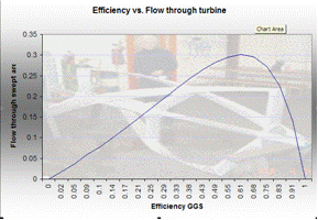
Figure 1. Relationship between flow through an axial turbine and efficiency (pictue from (9):

Further assumptions include:

The ‘sphere of influence’ displayed by each turbine is towards the upper permitted regions, as the flow rate is generally brisk in suitable generating sites, at 5 times the radius of the structure, when considering transversely deployed turbines, that is, perpendicular to the flow (8).
This effect is cumulative, as would be expected, adding two portions of highly turbulent fluid to each other will not cancel out the turbulence as each cannot display an exact opposite phase per se; uncertainty promulgates towards different turbulence characteristics as by its nature turbulance is non-symmetrical (7)(11).
Though the turbulence wake model produced predicts the effective ‘spread’ radius downstream, the additive blockage effects lead to an increase of backwater: a manifestation of localised head difference across the extraction site (6). Since, therefore, the wake model suggested that lateral packing densities can be relatively large, it must be regarded in conjunction with the blockage effects (7). In open channels, according to RGU, the backwater effect (figure 2.) is not as significant as in tidal estuaries or sea lochs, where this can actually increase the power extraction potential due to something of a damming effect, and the SIF could be as much as 50% in such sites, (2)(5).
Model flow is an average bulk flow rate, i.e., assuming a linear velocity profile, thus flow velocity can be validated using the velocity profile model against flow rates given on hydrographic charts.

To facilitate the comparison of the effects of varying turbine deployment on the flow regime, with regards to the SIF, the input data used was the output data predicted by the tidal velocity calculation model. Two different versions of the model were created, one that can compare three different deployment configurations, for instance, a linearly increasing deployment; and the second model allows a user to compare many different combinations of different turbines to assess which is the most proficient operator at a given site. The latter model may be used specifically for the last stages of the technology methodology, in conjunction with a parametric economic model, as the turbine configuration that generates the most power in a given space may not have the shortest payback time as the market develops through its infancy. It is likely that it may mirror that of the wind turbine market, with a clear ‘winner’ emerging as the industry favourite. At this time economic predictions will be grounded in clear patterns and discernable scaling factors. For more information on this please see economics/methodology section.

Figure 2. – Velocity and head changes in a channel at the point of extraction (9)

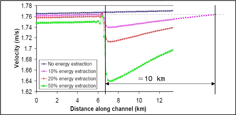
Figure 3. – Velocity reduction at extraction point and distance to free stream rejuvenation (modified (9)

The Model

To model the SIF, Microsoft Excel was used, rather than CFD for example, as the latter approach would have been outwith the reasonable bounds of time permitted for the investigation. Once a site was selected and average spring and neap velocities were calculated, the tidal variations were approximated by a visual Fourier analysis. The tidal cycle was divided into increments of 5 minutes to provide a sufficient resolution for further calculations. As the velocity can then be calculated for any point in the tidal cycle, the kinetic energy flux available can also be found. Thus by using the energy capture equation for turbines, and subtracting the result from the net energy available, the resultant net velocity reduction can be calculated. This applies because of continuity, that is, the mass of the body of water (treated as an incompressible fluid) cannot change, so if a portion of the kinetic energy of the water is removed, the velocity must decrease proportionally to the square of the velocity. As one might expect, the overall effect of a single turbine is marginal, but as subsequent turbines are added to the channel, and the flow velocity is sequentially altered, there comes a point where the subsequent addition of turbines actually will have an adverse effect on energy capture. This is also due to the additive effects of blockage, described by the Manning correction factors and the sphere of influence exerted by each turbine.

By calculating the percentage reduction of the nominal flow for each turbine deployment configuration, the SIF can be seen. Similarly, the effective horizontal component of gravitational attraction can be calculated, and the work done on the body of water, and how this force relates to the increased friction in the channel caused by the level of blockage and increased turbulence. The complexity however of turbulent flow means it is difficult and involving to model the return to free stream velocity, thus, as an initial attempt to investigate possible rejuvenation distances, a simple method was devised. The effective gravitational attraction was used to find the acceleration on the body of water at each timestep, the duration of the force and hence, the net downstream rejuvenation distance. As such, it is difficult to validate this data, but it is in general accord with RGU data in figure 3, but the theory is admittedly simplistic, and may be open to error.

Theory:

The cyclic pattern for tidal velocity can be approximated by the following function, where the input velocities (average maximum spring and neap tides) are taken from the tidal velocity calculation model:

Cyclic sinusoidal function: , 1

where 2

and T is taken as 745 minutes. It is assumed that there is little difference in the generating capacity between ebb and flood tides (when calculating SIF - not necissarily true), and t is any time in which we are interested, and has been calculated in the excel model in five minute intervals for a full cycle.

Turbine power is given by: 3
where C_P (power coefficient), and A (area), can be defined by the user. By applying the equation to the velocity at each 5 minute timestep, it is possible to determine the energy extracted over a full cycle, and consequently, for the year.

The kinetic energy flux in a channel can be found by the following equation; 4

which shows the energy flux is proportional to the cube of the velocity. Since the dimensions of the channel and the velocity are known, the kinetic energy of the body of water can be found at any time. Similarly, since the change of velocity of the body of water can be seen between successive time periods in the spreadsheet, the average acceleration of the body of water can be calculated at each timestep, thus the average effective horizontal component of the gravitational force can also be calculated based around N2, (12)(13). To interpolate possible rejuvenation distances, the effective force after extraction and thus the work done on the body of water can be used in conjunction with simple equations of motion to calculate the return to free stream velocity, though as discussed, this is very simplistic, and it is difficult to validate the accuracy of this method, (12)(14). The underlying postulation is that gravitational forces and viscous shear interactions may return the molecules to the free stream velocity after sufficient time has elapsed. If it proves to be the case that this method is indeed overly simplistic, a dedicated turbulent wake program that was also developed can be used instead, and is available from the tools section of the website, however it is constrained by fairly basic vorticity and actuator disk theory. Perhaps, as a further area of development, the dedicated model could be integrated into the SIF model.

Conclusions

The modelling exercise has raised some interesting points, and some that are not easily resolved:

Continually adding turbines/energy extraction mechanisms to a tidal stream reduces the collective net performance, such that each successive unit is increasingly less efficient at energy extraction, until a point is reached where generation is adversely affected. Thus, a lateral multi-turbine deployment should be optimised for the induced flow reduction caused by their presence in the tidal stream, whether that is in terms of rated capacity or indeed, cut-in velocity.
SIF constraints should be noted, as it is likely that they may form legislation at some point.
It is unlikely that the SIF could be reached at every given cross section due to topographic conditions and space/depth constraints however, so the approach to SIF limitations (10% flow reduction in the modelled site) should be taken into consideration. For example, as the net flow rate will be less than the free-stream velocity for a certain distance downstream, placing energy extraction devices very close to the first ‘row’ will mean the SIF at the second cross section will be approached more quickly, as the entrance velocity is already diminished. Therefore, it may be beneficial to place the turbines/devices slightly further downstream to maximise their efficiency. Perhaps this will be a balance between infrastructure costs and generation capacity. If however the SIF cannot be reached at the cross sections of the channel, then perhaps the 250-1000m suggested longitudinal packing density (15) will be sufficient.
For staggered downstream deployment, i.e., minimal wake interaction between successive turbines, perhaps a denser packing density would be optimal, as long as net energy extraction does not exceed the limits.
If topographic constraints limit deployment potential, perhaps smaller venturi type turbines would be the most beneficial, as any extraction below the SIF is in essence, waste. Technology is still emerging but studies have been done on shrouded and diffuser augmented turbines, with promising efficiencies of up to 3 times the Betz limit. In diffuser augmented turbines, sometimes slats are placed in the diffuser to allow boundary layer reenergising. Similarly, it has been suggested that placing the generator coils in the outer race of a shrouded turbine may reduce complexity, as the gearbox is effectively removed. These variant technologies may suit compliance with SIF conditions and the economic balance, if they are proved to be viable technologies.

Further work

There seems to exist a relationship between the percentage of the cross section area of a channel that is occupied by the swept area of extraction devices and the significant impact factor. It is not quite linear, and hence site specific, but could, upon further investigation, form the basis of a very useful boundary condition for potential developers to assess quickly the likely SIF, site feasibility and economic viability This will likely be a function of flow velocity, total swept area, relative turbine permeability at maximum efficiency and of course, turbine efficiency itself.

References

1	CHRISTIANSENA, M. and HASAGERA, C., Risø National Laboratory, ISPRS: Wake Studies around a Large Offshore Wind Farm Using Satellite and Airborne Sar. [PDF] 2005 [cited 03 May 2006]; Available from http://www.isprs.org/publications/related/ISRSE/html/papers/272.pdf
2	Black & Veatch Ltd., The Carbon Trust: Phase 1 & 2 Uk Tidal Stream Energy Resource Assessment. [Webpage] 2005 [cited 02 May 2006]; Available from http://www.thecarbontrust.co.uk/ctmarine10/page4.htm
3	DTI, The Robert Gordon University: A Scoping Study for an Environmental Impact Field Program in Tidal Current Energy [ETSU T/04/00213/REP; DTI Pub/URN 02/882]. [PDF] 2002 [cited 03 May 2006]; Available from http://www.dti.gov.uk/renewables/publications/pdfs/t0400213.pdf
4	BBC: Warning over Tidal Energy Impact. [Webpage] [cited 03 May 2006]; Available from http://news.bbc.co.uk/1/hi/scotland/3580484.stm
5	COUCH, S. and BRYDEN, I.G., Supergen Marine Marec Paper: The Impact of Energy Extraction on Tidal Flow Development. [PDF] 2004 [cited 03 May 2006]; Available from http://www.supergen-marine.org.uk/documents/papers/Public/Resource%20Estimation/Marec_2004_Couch_Bryden.pdf
6	CHARBENEAU, R., et al., US Dept. of Transportation: Backwater Effects of Piers in Subcritical Flow. [PDF] 2001 [cited 02 May 2006]; Available from http://www.utexas.edu/research/ctr/pdf_reports/1805_1.pdf
7	CHOW, V.T., Open-Channel Hydraulics. Mcgraw-Hill Civil Engineering Series. 1959, New York, London: McGraw-Hill Education. pp. 692. ISBN 007085906X.
8	ARCEMENT, G. and SCHNEIDER, V., USGS Water-supply Paper 2339: Guide for Selecting Manning’s Roughness Coefficients for Natural Channels and Flood Plains, 1989 United States Geological Survey
9	GORBAN, A.N., et al., Limits of the Turbine Efficiency for Free Fluid Flow. Transactions of the ASME Journal of Energy Resources Technology, 2001. 123(4): p. 311-17.
10	THAKE, J., DTI Renewables: Development, Installation and Testing of a Large Scale Tidal Current Turbine. [PDF] 2005 [cited 02 May 2006]; Available from http://www.dti.gov.uk/renewables/publications/pdfs/t060021rep.pdf
11	COPELAND, G., Seminar on Turbulence Modelling. 2006, University of Strathclyde.
12	BOWDITCH, N., The American Practical Navigator Chapter 9: Tides and Tidal Currents, and Nautical Charts. [cited 02 May 2006]; IRBS Available from http://www.irbs.com/bowditch/pdf/chapt09.pdf
13	HANNAH, J. and HILLIER, M., Applied Mechanics. Longman Scientific & Technical. 1995, Harlow: Longman. pp. 448. ISBN 0582256321.
14	CENGEL, Y. and BOLES, M., Thermodynamics: An Engineering Approach. Mcgraw Hill Higher Education. 1989, New York, London: McGraw Hill. pp. 867. ISBN 0071250840.
15	Garrad Hassan, Scottish Executive: Scottish Renewable Resource 2001– Volume 1 - Analysis. [PDF] 2003 [cited 03 May 2006]; Available from http://www.scotland.gov.uk/Resource/Doc/47176/0014634.pdf Garrad Hassan, Scottish Executive: Scottish Renewable Resource 2001–Volume 2 - Context. [PDF] 2003 [cited 03 May 2006]; Available from http://www.scotland.gov.uk/Resource/Doc/47176/0014635.pdf

MARINE CURRENT RESOURCE AND TECHNOLOGY METHODOLOGY

Environment: Significant Impact Factor (SIF)