• Theory
  • Introduction
  • BEM Theory
• Available BEM Codes
• Code Modifications
  • Modifications
  • Code Operators
  • Code Interface
• Adding Profiles
  • Blade Profile Design
  • Multiple Profiles
  • Additional Profiles
  • Adding Own Profile
  • Modelling Degradation
• Methodology
  • Systematic Study
  • Geometry
• Results
  • Introduction
  • Uniform Pitch Result
  • Twisted Blade Results
  • Hub Radius Results
  • Increasing Tip Radius (Maintaining Uniform Chord)
  • Increasing Tip Radius (Twisted Blade)
  • Blade Position Results
  • Chord
  • Taper
  • R.P.M.
  • Variable Profiles
  • Number of Blades
  • Contra Rotation
• Tools
  • Tools Intro
  • Xfoil
  • Rfoil

Momentum Theory

 

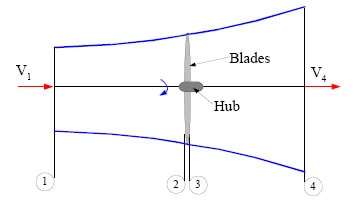
Figure 1

Figure 1 displays a stream tube around a MCT with four stations marked to indicate the regions upstream (1) within (2 and 3) and downstream (4) of the rotor. Energy is extracted from the water between regions 2 and 3 and a change in pressure is experienced.
Making the assumptions below we can apply Bernoulli’s Equation to define the force on the water in the axial direction, remembering that force equals pressure time’s area:

1. Flow is frictionless between 1 and 2 and between 3 and 4
2. and
3. Axial induction factor (quantifies the degree to which the water slows down as it passes through the rotor in the axial direction)
4. and

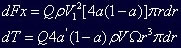
For an element of fluid, the axial force is then defined as: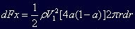

Now consider the rotational annular stream tube shown in Figure 2. As the water passes between stations 2 and 3 the motion of the turbine causes the water to rotate in the blade wake.

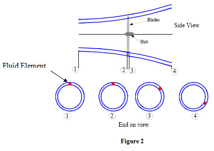
Applying the conservation of angular momentum to this annular stream tube, noting that the blade wake rotates with an angular velocity and the blades rotate with an angular velocity of Ω, we can define the torque (tangential force) for a rotating annular element of fluid as:

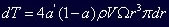
With representing the tangential induction factor.

We therefore have two equations from momentum theory which represent the axial and tangential force on a fluid element.

Blade Element Theory

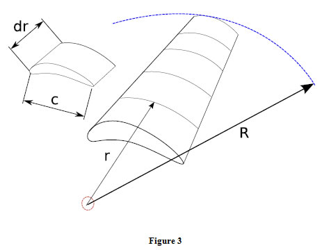
Blade element theory involves splitting the blade up into N elements as shown Figure 3 below. Each element will experience varying flow characteristics as they have differing rotational speeds (Ωr) and depending on the design, a differing chord (C) and twist distribution . The theory calculates the relative flow at each section and determines the overall performance characteristics by integrating along the span of the blade.
Two vital assumptions are made when applying blade element theory:

1. There are no aerodynamic interactions between the different blade elements.
2.  The forces on the blade elements are only determined by the lift and drag coefficients.

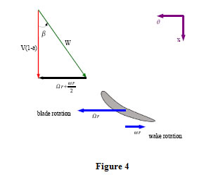
The lift and drag coefficients will vary for each aerofoil design. CL-α and CD-α curves can be obtained from experimental data, however many of these tests are performed on stationary, non-rotating aerofoils. It is therefore necessary to define a flow relationship between a rotating aerofoil and a stationary test. Figure 4 displays the flow into a turbine blade. With the blade rotating with a speed Ω and the flow exiting the blade rotating with a speed , an expression for the average tangential velocity that the blade experiences can be deduced as:

Making the following assumptions:

1. 
2. Tip speed ratio =

We can deduce an expression for the inflow angle between the incoming flow velocity , and the average tangential velocity described above:

This will vary for each blade element as it is dependant on the radial position of the element (r).

From figure 4 we can also determine an expression for the resultant velocity W between the local inflow and tangential velocities:

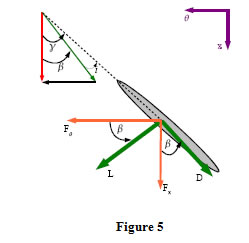
The forces each blade element experiences are displayed in Figure 5.  Lift (L) and drag (D) forces are perpendicular and parallel to the oncoming flow. For each blade element the axial (Fx) and tangential forces (Fθ) can be defined from Figure 5 as:

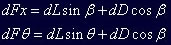
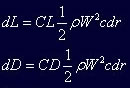
 and   can be obtained using experimental definitions of the lift and drag coefficients for an aerofoil and expressed as the following:

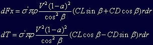
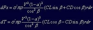
Combining the above two sets of equations and making the following assumptions:

1. B = number of blades
2. Torque on an element equals tangential force multiplied by radius
3. Local blade solidity  

We can deduce a set of equations for the axial thrust and torque on a (B) number of blades rotor as follows, (expressing  and  in terms of induction factors):

Tip Loss Correction Factor

Due to vortex effects at the blade tips, an expression for the incurred losses along the span of the blade needs to be factored into the analyses. In BEMT a tip loss correction factor Q is introduced, which varies from 0 to 1 where the magnitude determines the reduction in forces along the blade.

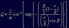
This can then be applied to the equations defined by momentum theory for the axial and tangential forces on a fluid element:

Blade Element Momentum Equations

Combining momentum and blade element theory, we now have four equations, two which represent the axial thrust and torque in terms of flow parameters:

And two which represent axial thrust and torque in terms of the blade sections lift and drag coefficients.

Rotor Performance

The rotor performance can then be determined by performing a momentum balance of the blade element momentum equations. This produces the following two relationships:

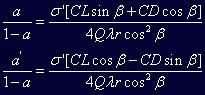
These relationships are used in an iterative process to determine the induction factors along the span of the blade and are primarily used in the blade design procedure.
By integrating the contribution to the power output by each rotating annulus along the span of the blade we can determine the total power output from the rotor:

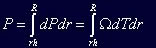
Where: rh hub radius

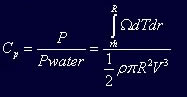
The power coefficient can then be determined by:

Reference:

www.dur.ac.uk/g.l.ingram/download/wind_turbine_design.pdf