• Theory
  • Introduction
  • BEM Theory
• Available BEM Codes
• Code Modifications
  • Modifications
  • Code Operators
  • Code Interface
• Adding Profiles
  • Blade Profile Design
  • Multiple Profiles
  • Additional Profiles
  • Adding Own Profile
  • Modelling Degradation
• Methodology
  • Systematic Study
  • Geometry
• Results
  • Introduction
  • Uniform Pitch Result
  • Twisted Blade Results
  • Hub Radius Results
  • Increasing Tip Radius (Maintaining Uniform Chord)
  • Increasing Tip Radius (Twisted Blade)
  • Blade Position Results
  • Chord
  • Taper
  • R.P.M.
  • Variable Profiles
  • Number of Blades
  • Contra Rotation
• Tools
  • Tools Intro
  • Xfoil
  • Rfoil

How to add your own profiles to the code

In the BEM programme, different aerofoil profiles are represented by their 2-dimensional lift and drag characteristics in an individual subroutine for each aerofoil shape. In order to input a new profile, you will first need lift and drag polars. These can either be obtained from experimental data or if experimental data is unavailable, lift and drag coefficients can be calculated using a program such as XFOIL.

XFOIL is an open source panel solver developed by Professor Mark Drela at MIT which can calculate lift, drag, pressure and pitching moment coefficients for a given cross sectional geometry and angle of attack (AoA). This can be done for a sequence of AoA and the results output to a file. For our study we used RFOIL for this purpose. RFOIL is a programme, based on XFOIL, which has been modified at TU Delft in the Netherlands. RFOIL can provide solutions more concurrent with experimental data, particularly around stall.

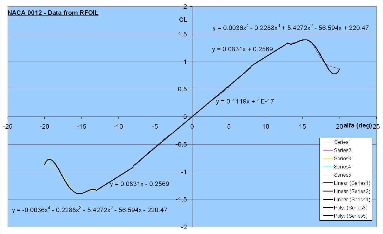
 Using a spreadsheet programme, such as Excel, these results can be graphed and used to create a set of polynomials describing the aerofoil characteristics. These polynomials can then be used to create a subroutine in the programme. See image below for a graphical view of how these polynomials were generated.

Steps:

1. Get a set of co-ordinates for the geometry of the desired aerofoil profile and save the file in the XFOIL directory.
2. (Aerofoil coordinate databases can be obtained from UIUC and AID)
3. In XFOIL, load the coordinate file.
1. LOAD
2. aerofoil_name.dat (example)
4. Specify a viscous boundary layer and chord Reynolds Number.
1. VISC
2. 1 500 000 (example)
5. Create a file to save outputs to.
1. PACC
2. output.pol (example)
6. Define a range of angles of attack to calculate over and the interval between values.
1. ASEQ
2. -25 (example)
3. 30 (example)
4. 1 (example)
7. Open output file in spreadsheet programme. (Data may require some formatting into columns.)
8. Graph CL vs. α and CD vs. α
9. Use trend-lines to get polynomials approximating curves. (Data may need to be separated into several curves.)
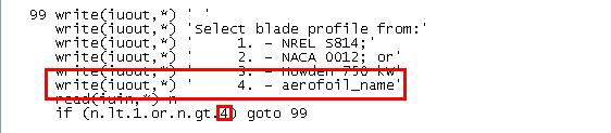
10. Insert polynomials into a new subroutine in the Fortran source code and add in references to new subroutine. (See images below.)

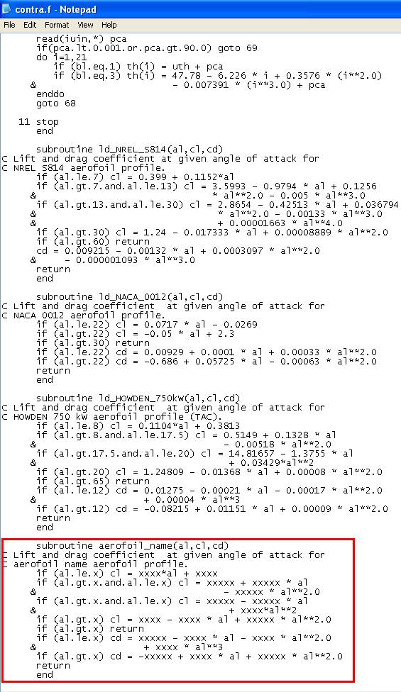
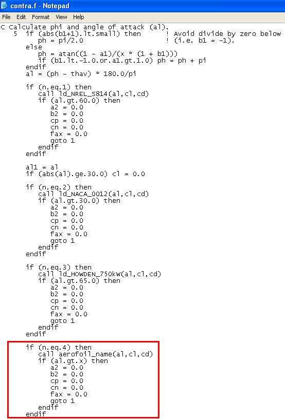
NB: The third revision to the source code occurs twice.