
 Home
Home 

Glauert's Blade Element Momentrum Theory
Actuator disk theory provides little information on rotor performance
or blade design. Blade element theory attempts to address this
by considering the effects of blade design ie. shape, section,
twist, etc. Blade element theory models the rotor as a set of
isolated two-dimensional blade elements to which we can then apply
2-dimensional aerodynamic theory individually and then perform
an integration to find thrust and torque.
First the control volume described in (Froude)
is discretised into N annular elements of thickness dr,
whose crossflow boundaries are those of the control volume, and
whose lateral boundaries follow streamlines (thus, as mentioned
previously, there will be no crossflow momentum flux between annular
elements).
The following assumptions are adhered to:
- Isolated elements – one element does not affect the others (no in-plane inflow)
- Force from the blades is constant through the annular element, consistent with an assumption of an infinite number of blades
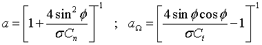
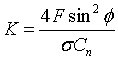
Assumption number 1 is only valid if the rotor is exactly perpendicular to the flow, ie. no yaw and even velocity distribution. A correction factor for CP in cases where yaw angle is not zero is given by
![]()
where ![]() is the yaw angle. The accuracy of this approximation is tenuous.
is the yaw angle. The accuracy of this approximation is tenuous.
Now consider an arbitrary spanwise location along the rotor blade. The rotor is rotating and hence there is a translational velocity, and there is also an inflow to the rotor disk.
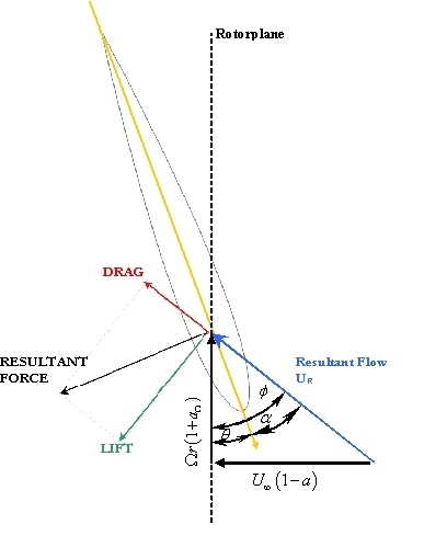
The rotor blade element, therefore, has lift and drag forces
L, D, and these generate thrust and torque, dT and dQ/r respectively
(T is thust, Q is torque, r is radial position of the blade element).
Hence we have a set of velocities, angles and forces as follows:
| the rotor disk induced velocity | |
| velocity due to rotation | |
| resultant hydrodynamic velocity | |
| local blade twist, the angle between the zero lift line to the blade translational velocity | |
| advance angle as given in equation (Froude eqn 31) | |
| hydrodynamic incidence |
These blade element properties are considered alongside the axial
momentum conditions as described by Froude, and the solution is
simultaneous, coupling momentum considerations with hydrodynamic
forces for actual blades. As before, the pressure distribution
along streamlines defining annular elements is assumed to give
no net force in the axial direction, and since the cross sectional
area of the annular element at the rotor plane is 2prdr we find
the integral momentum equation can be used with the definitions
of ![]() and
and ![]()
![]() and the assumption that the previously defined relation between
axial induction and inflow speed is still valid to be be calculated
as:
and the assumption that the previously defined relation between
axial induction and inflow speed is still valid to be be calculated
as:
 |
Eqn 1 |
Re-casting the moment of momentum equations (![]() ) into integral form and re-writing in a similar fashion:
) into integral form and re-writing in a similar fashion:
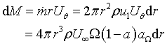 |
Eqn 2 |
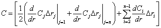
The left hand sides of these equations are calculated at the
blade element from flow conditions, and the right hand sides are
calculated from momentum considerations.
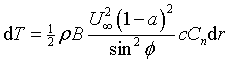
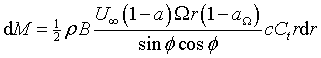
Thus for a blade element:
| Eqn 3 |
and resolving forces into and perpendicular to the rotorplane and normalising gives
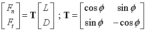 |
Eqn 4 |
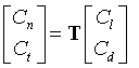 |
Eqn 5 |
Noting that Ft and Fn are forces per unit length the normal force and the torque on a c.v. of thickness dr are respectively
| Eqn 6 |
The local solidity of an anular element with B number of blades and local chord c(r) is
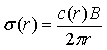 |
Eqn 7 |
and a geometric result from the above figure gives
| Eqn 8 |
Using these four relations we may write
 |
Eqn 9 |
 |
Eqn 10 |
If these and the previous identities for dT and dM are equated, the following expressions for the axial and tangential induction factors may be obtained:
 |
Eqn 11 |
In order that results are accurate, two corrections must be made: the first is to account for assumption 2 requiring an infinite number of infinitesimal blades and is dealt with by Prandtl’s tip loss factor, F, which is applied to equations 9 & 10, and when the derivation is carried out as before results in modified expressions for axial and tangential induction factors:
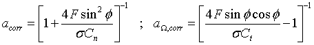 |
Eqn 12 |
where
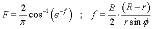 |
Eqn 13 |
The second correction is for the problem discusses in Froude where the momentum theory breaks down at high axial induction factors (a >~0.4). An empirical correction is proposed by Spera which states:
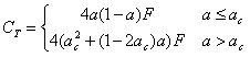 |
Eqn 14 |
with critical induction factor ac = 0.2 and F is the tip loss correction factor. It can be shown that for values of a below the critical, eqn 12 still stands, but when the axial induction is above the critical value the following relationship must be used:
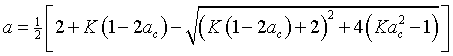 |
Eqn 15 |
 |
Eqn 16 |
Due to the somewhat circular nature of these expressions, and those from momentum theory, an analytical solution is not feasible and an iterative approach is required. An algorithm may be applied to each control volume in turn to calculate values of induction factors, and thus associated blade element parameters, which are then integrated. This iterative approach is time consuming if done manually, but is ideal for automation, and a Matlab script has been generated for such a purpose.
Thus the algorithm proceeds as follows:
-
Assume initial values for axial and tangential induction factors (e.g. a = a
 =
0)
=
0) - Calculate the flow angle f and thus local angle of attack a
- Read Cl(a) and Cd(a) from lookup table and compute Cn, Ct
- Calculate new induction factors from eqns 17 or 22 and 18
- Repeat until convergence of induction factors (or other parameters)
- Calculate blade element forces
It is unlikely that the thrust and torque calculations will result in convenient analytical expressions that can be integrated algebraically and in practise a numerical integration scheme is used viz:
 |
Eqn 17 |
For n blade elements of spanwise length ri for parameter
C.
The Euler turbomachinery equation states that power is simply
the shaft torque by angular velocity. So if M is calculated from
calculated values of Ft as follows and it is assumed
that all torque on control volumes is reacted by the blades we
have:
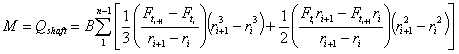 |
Eqn 18 |
And so ![]()
Results for the model run at different flow conditions are available in the results package here.
References & Bibliography
| 1 | HANSEN, M.O.L., Aerodynamics of Wind Turbines : Rotors, Loads and Structure. 2001, London: James & James (Science Publishers) Ltd. pp. 152. ISBN 1902916069. |
| 2 | BURTON, T., et al., Wind Energy Handbook. 2001, Chichester, New York: John Wiley and Sons Ltd. pp. 624. ISBN 0471489972. |
| 3 | MYERS, L. and BAHAJ, A.S., Power Output Performance Characteristics of a Horizontal Axis Marine Current Turbine. Renewable Energy, 2006. 31(2): p. 197-208. |
| 4 | BAHAJ, A.S., et al., Power and Thrust Measurements of Marine Current Turbines under Various Hydrodynamic Flow Conditions in a Cavitation Tunnel and a Towing Tank. Renewable Energy. In Press, Corrected Proof. |
| 5 | BAHAJ, A.S. and MYERS, L.E., Fundamentals Applicable to the Utilisation of Marine Current Turbines for Energy Production. Renewable Energy, 2003. 28(14): p. 2205-2211 |
| 6 | BATTEN, W.M.J., et al., Hydrodynamics of Marine Current Turbines. Renewable Energy, 2006. 31(2): p. 249-256. |
| 7 | LOFTIN, L.K. and BURSNALL, W.J., NACA TN-1773: Effects of Variations in Reynolds Number between 3.0x10⁶ and 25.0x10⁶ Upon the Aerodynamic Characteristics of a Number of Naca 6-Series Airfoil Sections, 1948 NASA Langley |
| 8 | KLIMAS, P. and SHELDAHL, R., SAND80-2114: Aerodynamic Characteristics of Seven Symmetrical Airfoil Sections through 180-Degree Angle of Attack for Use in Aerodynamic Analysis of Vertical Axis Wind Turbines, 1981 Sandia National Laboratories, Albuquerque |
Go back to Contents