HOMER Modelling Software
Why Homer?
It is important to define how the group went about testing, analysing and validating new configurations in our attempts to supply sustainable heating on Eigg. The primary software of choice was HOMER (Hybrid Optimization of Multiple Energy Resources).
Why?
Other types of software were available but the group concluded that HOMER was the most appropriate for the following reasons:
• There is an existing HOMER model for the Isle of Eigg’s microgrid(1)
• HOMER has access to extensive climate data files from around the world
• HOMER has a wide range of technologies and includes all those that are relevant to the project
• HOMER includes a cost analysis as part of its simulation
• HOMER is user friendly and it is possible to become proficient without much training
• HOMER has a strong support network and a large online community to help with any issues
• HOMER is free for a month’s trial and offers a significant student discount for each month thereafter
• HOMER has a history of being used in successful reports in various parts of the world eg. China (2) and India (3).
Homer files for the Eigg case study are available in the useful links section.
simulating with homer
Defining the Load
The first step in modelling any microgrid system is defining the load, both electrical and thermal. For the purposes of this project, two separate electrical loads were necessary - one for the current electricity demands and another for the heat pumps that are to be installed.
Electrical loads can be imported or made manually with timesteps of either a minute or an hour. As the project is investigating hypothetical future systems, a manual input was required. To do this, a similar method to Breen (2015)(1) was adopted whereby an inbuilt daily profile was chosen and then scaled as appropriate to represent the new system.
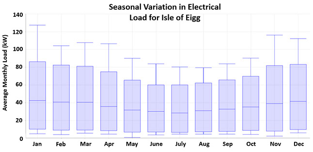
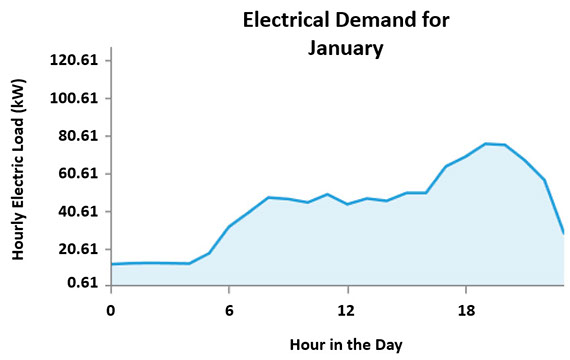
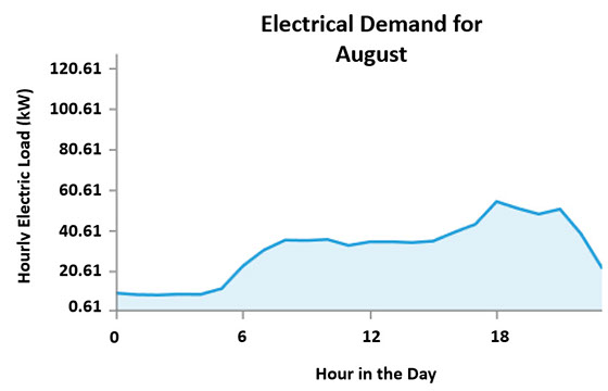
The daily profile chosen was that of a ‘community’. There is a peak in the evening but the afternoon is steady to represent the fact that most people remain at home during the day rather than commuting to work. This community profile is shown to the right for January and August. It is clear that both profiles are similar but January is scaled up. There is a day-to-day random variability of 10% defined in the model which is why the profiles do not match exactly. The seasonal profile is included by selecting a peak month which combines with the daily to produce a yearly profile with an hourly time step. The three graphs refer to the present electrical demand.
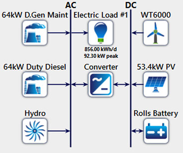
Daily profiles are then scaled by the average load throughout the year. Breen (1) found this to be 856kWh/day for the current electrical load. The heating loads for the present housing stock were estimated along with that of the housing after refurbishment (full details found here). Additionally, the electric loads for air and ground source heat pumps in both types of housing were calculated, as outlined here. Finally, the aforementioned electrical loads were modified to account for the inclusion of biomass into the final solution.
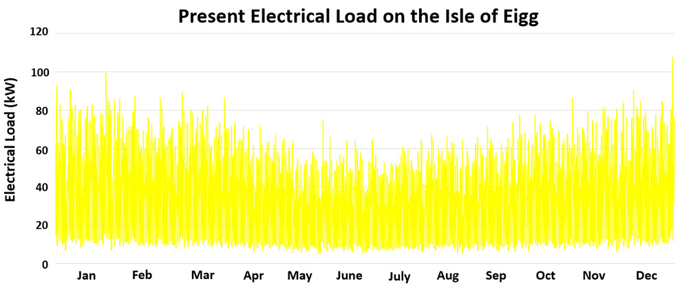
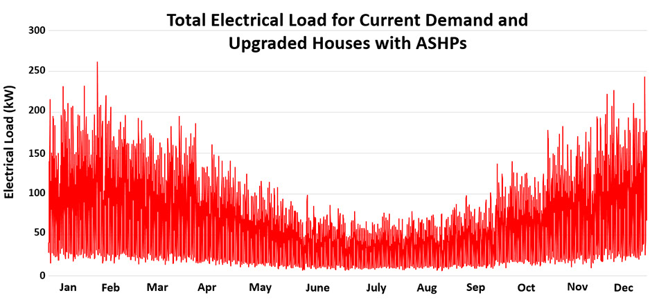
Below are the hourly profiles throughout the year for the pre-existing ‘normal’ electric load and, to give an example, that satisfying air source heat pumps in a scenario with upgraded houses (see section about upgrading houses here). The total load is simply the sum of them both.
Present Electrical Load
Electrical Load with Housing Upgrades and ASHPs
components
In HOMER the load and generation must match otherwise the simulation cannot take place. As such, generation components along with storage and converters (if wanted/needed) must be defined. An ‘autosize genset’ feature allows for HOMER to automatically match the predefined load with the most appropriate diesel generator size.
Many components are in-built to HOMER, including their capacity along with typical installation, maintenance and replacement costs, all of which can be edited as desired. It is very simple to input custom generation technologies so long as the required specification and data are available.
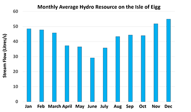
Resources
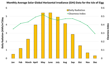
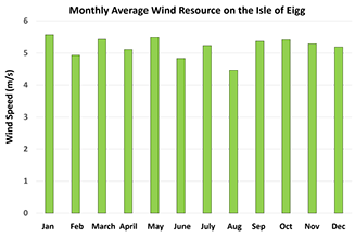
Renewable resources must be included before a simulation is possible. This is of course because renewable generation is dependent upon underlying meteorological factors (4). Solar, wind, hydro and biomass resources can all be input into HOMER to produce an output from the related technologies. Solar, wind and hydro resource data can be included manually or drawn from databases courtesy of various institutions such as NASA (5). In the case of Eigg, no local data exists to hand and so a synthetic data profile is calculated using an algorithm in order to represent Eigg. The following graphs show that there is a much larger solar resource in summer than winter whilst the opposite is true for hydro, which is provide for by rainfall. The wind varies but there is only a small increase on average from summer to winter.
ECONOMICS AND OPTIMISATION
The following section takes its information from Lambert et al (6).
HOMER performs a life-cycle cost analysis, taking account of all costs that occur during the lifetime of the project (as specified by the user). For this project, the life-cycle was set at 25 years and a discount rate of 8% was used. The discount rate reduces future cash flows back to the present.
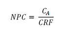
HOMER uses the metric of Net Present Cost (NPC) to evaluate different systems. This value accounts for all costs and revenues throughout the project lifetime including capital, operation and maintenance, replacements, fuel and pollution penalties. Costs are assigned positive values and revenues negative and so the NPC is equal but opposite to the Net Present Value (NPV).
The NPC is the ‘economic figure of merit’ and is the principle optimisation metric for which HOMER bases the optimal system solution. It is calculated using standard risk management formulation:
eq1
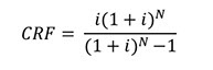
Where 𝐶𝐴 is the total annualised cost and CRF is the capital recovery factor defined as:
eq2
Where 𝑖 is the annual real interest rate and N is the number of years.
The user can decide whether the NPC remains as the primary optimisation factor or whether another metric, economic or otherwise, is more important.

© University of Strathclyde | TEC Eigg | Sustainable Engineering 2016