Appliances | Space Heating | Hot Water | Comparison

Demand

Space Heating

Once we finished our study about which would be the best material that we could install in our cabins in terms of energy saving (space heating + embodied energy) choosing TIMBER FRAME as the ideal option, we used ESP-r again to calculate the real space heating demand that we will have in our case study. It is important to highlight that in the previous simulations run to choose the best material, the occupancy was assumed to be constant within the year due to we only wanted to pick the best material by having a look to its performance (kWh). However, now we want to predict the exact space heating demand that we will have in our site and climate and occupancy will be the most sensitive parameters.

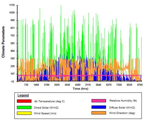
Climate

Database from Eskdalemuir Seismological Recording Station which is about 10 km far from Craik was imported to ESP-r. It has useful information data such as dry bulb temperature, diffuse solar on the horizontal, direct normal solar intensity, wind direction, wind speed and relative humidity.

Climate Data

Occupancy

We could not use the number of days per week that each cabin will be occupied in a weekly basis due to constraints on ESP-r software. In ESP-r we cannot run a simulation specifying that only some of the days within a week the cabin will be occupied (e.g. we cannot say that our cabin will be 4 days occupied per week). We have to assume constant occupancy and hence we run one simulation per month using the average people per cabin during a month. (e.g. an average of 5 people per cabin in May). Note that any other approach would have been difficult to implement due to the necessity of having a half hourly profile basis throughout the year in order to be able to export it later to Merit software and work in the supply-demand match.

It is important to highlight that, due to the occupancy approach carried out, casual gains for different levels of occupancy must be taken into account. Different number of people in a cabin will influence in the casual gains emitted and hence in the space heating demand. These casual gains were based on the behavioural models already explained in other sections of the website. Thus, it will be necessary to change and adjust the heat gains for each of the 12 monthly simulations that we run basing it on the occupancy. They were assumed to be the same during weekdays and weekend considering we are on a holiday accommodation and people have the same behaviour during the whole week.

Occupancy Heat Gains

100 W of sensible gains and 30 W of latent gains per person during occupied hours.

Lighting Heat Gains

8 CFL of 20W working when people are at home.

Equipment Heat Gains

These were the largest heat gains. They are linked with the heat emitted by the appliances. In order to calculate the heat gains, we used our own Excel spreadsheet of appliances uses (see appliances section), which takes into account the different behaviour models in terms of time and length of using of the equipment, and we changed the electricity consumption of the appliances for their heat gains emission. Heat gains values were taken from the ASHRAE Research Project 391-RP (see references section). Note that the appliances might work for a period less than one hour and ESP-r minimum input heat gains period is one hour so we must be careful with the values used and scale them down if it is required. Also note that if heat gains values of two or more consecutive hours are very close we took the average value of them and we set a heat gain period larger than one hour.

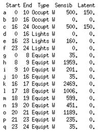
Heat gains for 5 people occupancy in a typical behaviour

The basic heating control used in the simulations was the following:

It starts working at 8am and it stops at 11am when people is supposed to leave the house to do some outdoors activities. It starts again at 3pm in case they come back early. It is switched off at midnight.
Set points 20 C for heating and 27 C for cooling. However cooling requirement was neglected due to Craik is located in Scotland and natural ventilation by opening the windows should be enough to cool down the cabin in summer.
Same control over the whole week. We are dealing with a holiday accommodation where people will tend to have the same behavioural schedule within the week. In the case that they stay at home some days we still have the same control due to some constraints in ESP-r that make difficult to change this control for each days when the behavioural model is not the typical one. Thus, the control could be assumed as a central heating control.

Simulations

Once all the necessary parameters were specified in ESP-r, the previously mentioned 12 simulations (1 per month) were run changing the casual gains from month to month according to our occupancy level study, e.g. January 3 people on average, February 2 people on average, etc. (see occupancy section for further details).

It should be also mentioned that we run sets of 12 simulations.Each set corresponds to a different behavioural model: Always at home, Typical scenario and Outdoor more. As we have all the results in a half-hourly basis, we could combine the data of these different behavioural models as we want in order to build a new more realistic model for a group of cabins which takes into account the possibility of having different behaviours on each cabin. For instance, for our case study in Craik, which first phase is composed of 6 cabins, we could built a model with a 3-2-1 combination, i.e. 3 families with 'Typical' behaviour, 2 with 'Outdoor' behaviour and 1 with 'At Home' behaviour.

The next table summarizes our findings:

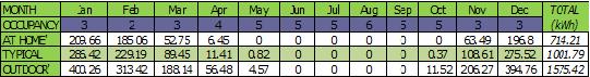
As we can see, assuming the same behaviour during the year, 'At Home' behaviour will have the total lowest demand and 'Outdoor' behaviour will have the highest as we predicted. Note also that the highest heating demand is concentrated on winter months and that from June to September we do not need heating in any of the models due to the good weather and the good insulation we have in the cabins. Moreover, in 'At Home' behaviour we do not need heating in May and October either due to the good insulation and the increase in the casual gains related to being all the day at home.

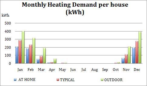
The following chart shows an annual graphical comparison between the three different behaviours.

And the monthly space heating consumption for the previous the previously mentioned 3-2-1 combination would be the following:

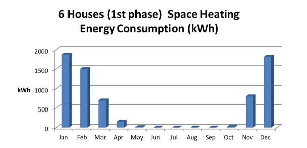
Monthly space heating consumption for Phase 1

The total monthly space heating energy consumption for the 6 houses would be 6,870.42 kWh, and hence the average consumption per house would be 1,145.07 kWh.