Approach to Validation

ESP-r as a building modelling software, has never before been utilised for district heating modelling. It was therefore vital as part of the development process of the software, to validate the development work done with real data.

Having large amounts of data available from the West Whitlawburn site allowed direct comparison with the model simulation results for empirical validation. Data measured at the site, such as flow rates, flow and return temperatures and heat input, are found to be either time-averaged values or a time series, allowing both quantitative and qualitative comparison.

To validate the working model, simulations were run for five varying months across the year in order to catch seasonal performance, using realistic demand profiles that were fed into the loads. In order for the simulations to show validation the model must respond to the demand similarly to that of the West Whitlawburn system in the parameters that are not actively controlled, both quantitively and qualitatively.

Analysis

Controlled Parameters

In order to make sure the model was accurate, the model control parameters were manipulated to match that of the average monthly flowrate, outflow and return temperatures of the monitored data to within 5% for the flowrate and 3°C for the temperatures. Figures 1-3 provide a comparison of these system parameters between the modelled and monitored data over two days of operation in December.

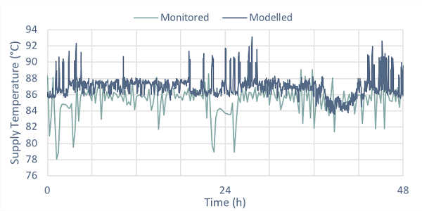
Figure 1: Supply Temperature Comparison

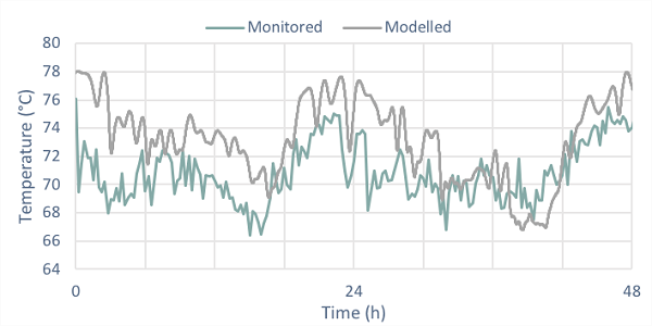
Figure 2: Return Temperature Comparison

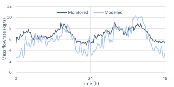
Figure 3: Mass Flow Rate Comparison

It is evident from Figures 1 to 3 that the model captures the overall daily operation of the district heating system, displaying distinct evening peaks and nighttime troughs in both the mass flow rate and return temperature. While the supply temperature remains constant to within an average of 2% of the actual flow. There are differences between some the two plots as well but these can be ascribed to the fact the model does not consider pressure, that the system is 'ideal' and that the control logic is fairly simplistic. This level of agreement between the controlled model parameters and the monitored data enables an investigation into the non-actively controlled parameters to be undertaken.

Performance Metric: Thermal Store Temperature

The performance metrics being assessed for validity, and not being actively controlled, were chosen to be the thermal store mean temperature, average heat input and buried pipe losses. The thermal store mean temperature was chosen due to the important role it plays in balancing supply and demand in both the West Whitlawburn system and in the model.

Table 1: Thermal Store Mean Temperature Monthly Comparison

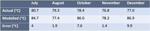
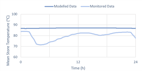
Figure 4: Thermal Store Mean Temperature Comparison

It is evident in the results from these simulations that across all 5 simulated months the thermal store was under-utilised in the model, as stressed in the higher average temperature in Table 1. Qualitatively this is backed-up in Figure 4, clearly showing that the model is not responding to the daily operating patterns during this time frame. This is due to the setting of the control parameters for the pumps and the fact the store is balancing the flows. An improved system would apply active control in order for the store to charge and discharge, depending on a set condition, and not simply the relative mass flow rate. This setting, however would require new control and bypass pipes to balance the flows.

Performance Metric: Boiler Heat Input

Similar demands at West Whitlawburn and in the model should require the same amount of heat energy inputted into the system over the month, and so the difference between the two, in terms of the average heat input, was investigated.

Table 2: Heat Input Monthly Comparison

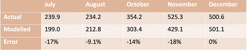
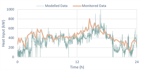
Figure 5: Input from Boilers Comparison

Simulation results showed that the average heat input in the system was consistently lower than that of the real system, with the maximum difference being out by 18%. The degree of change, however, can be explained by the omitted loads not included in the model. Qualitatively the model follows a very rough pattern to that monitored. Further analysis of the average heat input should be conducted using accurate demand data from the omitted loads, in order to understand the average heat input difference further, and the impact the omitted loads have.

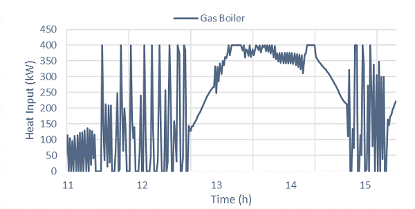
Figure 6: Numerical Instability in Heat Input

Yet the model results do show numerical instability when viewing the boilers individually, highlighting potential for future work. Figure 6 reveals the true nature of the gas boilers numerical instability, displaying between 11:30 and 12:30 the boiler repeatedly switches itself on and off, before recovering for a period of time and then slipping into instability once more. This is believed to be due to the control of the plant side flow rate in combination with the lag of the boiler PID controller. Future development of the module could be designed to include combustion and interactions with the internal heat exchanger.

Performance Metric: Buried Pipework Losses

If the model was modelled correctly then the system should remove similar amounts of heat from the system to that of real life system. Using the block meter data from the site a heat loss investigation was conducted to allow the simulations results to be compared to that of the values found in the investigation.

Table 3: Buried Distribution Losses Comparison

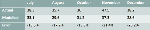
Simulation results showed that the difference between the model and the site in terms of buried heat losses ranged between 13 and 25% below that of the real system. In developing of the model, real life defects such as those that would exist with imperfect insulation were not modelled and there is a degree of uncertainty with the accuracy of the manipulated demand profiles. These facts will play a role in the difference between the two values.

Out with the results shown, further investigations were conducted to determine the impact of the return temperature and flow rate on the distribution losses. Interestingly the investigation showed that the distribution heat losses are relatively independent of return temperature and mass flowrate in the distribution network. The results of this allow a better understanding of the model, by showing that when the flow rate and return temperature are changed independently the other parameter adapts to counter the change. For example, when the return temperature increases the corresponding flow rate decreases through the control logic and this means that approximately the same amount of heat is circulating through the distribution network in both cases.

Discussion

Overall, the simulations showed promising results for a first attempt of validation. The response of the model captured the fundamental operation of the system, as shown in Figures 1 to 3. Quantititvely the model results are fairly accurate. The disagreement is not out by any order of magnitude and there are potential explainations for all the differences. The distribution losses are under estimated by 10-25%, this could be for numerous reasons such as omitted loads and unaccounted losses. Additional potential factors contributing to the difference in distribution losses include: uncertainties in regard to the demands that were artificially created, unaccounted components such as the thermal store, uncertainties regarding the ground temperature and improper insulation.

Improvments to this model could be made by revising the control routines used and capturing the control of the West Whitlawburn system more closely. Further site visits and data gathering should be conducted along with on-going correspondence with the site in order to gain a deeper understanding of the control methods used on site. Furthermore, more work is required in order to fully validate the model. Real demand data from individual blocks must be obtained and simulated using the data, to bring the model closer to validation. This also includes the terraces, as well as demand data from the omitted loads and simulated across a full year.