The Heating Network
The district heating network provides hot water and space heating to the ~550 terrace and tower properties. The system replaced electrical storage heaters and aimed to reduce the residents’ energy bills and improve the co-operative’s carbon footprint. The plant is housed in the Energy Centre and comprises a 740kW biomass boiler (#1 in Figure 1), 3 backup 1300kW gas boilers (#2), a 50m³ thermal store (#3) and meters for fuel consumption, heat input/output, mass flow rate and supply/return temperatures (#4).
Buried distribution pipes carry the heat to each block and a heat meter measures the cumulative heat delivery into that block (#5). Heat is then transferred through internal pipework. A Heat Interface Unit (HIU) is located in each dwelling which uses heat exchangers to produce water for space heating and domestic hot water. The HIUs (#6) monitor the total heat consumed by the property. Each dwelling is also equipped with a Smart Meter (#7) which controls the heating system and provides information on the resident’s energy usage. The system operates at supply temperatures of 85°C.
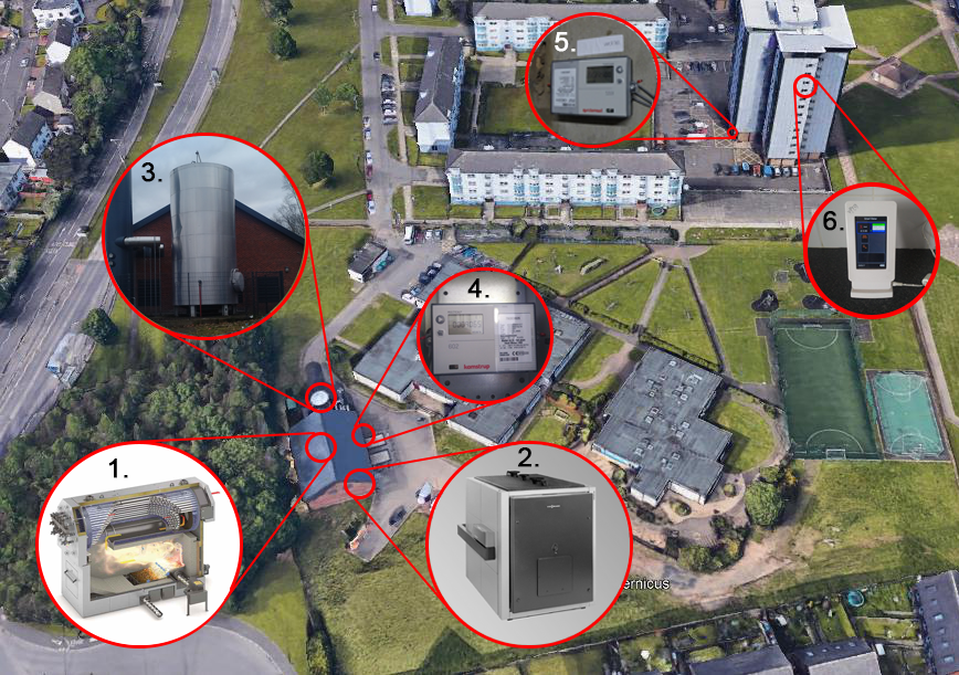
Figure 1: DHS Components and Layout
Carbon Footprint
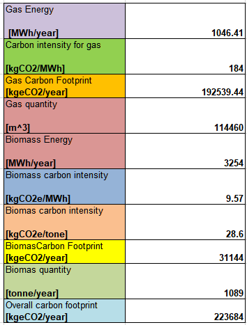
Heat policy takes into account the carbon footprint of different heating technologies. The Carbon Footprint is calculated by multiplying annual usage of energy by the carbon intensity of the energy. Different fuels emit different amounts of CO2 per unit of energy produced. West Whitlawburn uses gas and biomass boilers to supply the heating network and the footprint was calculated for each of these fuels. The sum of these gives the total operational carbon footprint of the district heating system.
The system is well monitored and data from meters installed in the boilers allowed the calculation of energy produced and fuel consumed for each. Gas fuel has a fixed carbon intensity that was assumed to be 184 kgCO2/MWh. When considering emissions resulting from biomass combustion it is necessary to take into account not only emissions from burning the fuel but also emissions resulting from the preparation and transportation of the fuel to the site. For the calculation, the Carbon Footprint Calculator was used (DECC B2C2). The default fuel chain was taken which includes 6 stages of the fuel life cycle, as shown in Figure 2.
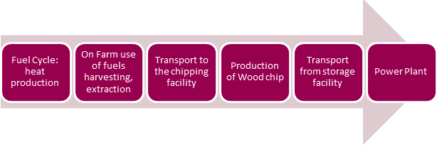
Figure 2: Biomass fuel supply chain
Table 1: Carbon Footprint Results
Operation
The operation of the West Whitlawburn system over the course of one day is provided graphically in Figure 3. Beginning in the early hours of the morning the biomass boiler charges up the thermal store until 5:30 am, at which point it begins to deplete for the next 2 hours to meet the morning demand of the residents. As the thermal store nears the practical minimum supply temperature of the district heating system the biomass boiler switches back on to replenish the thermal store. The gas boiler is used occasionally to top up the thermal store as seen in Figure 3 switching on to 70% capacity to meet the remaining load. This is due to the slow start up of the biomass boiler.
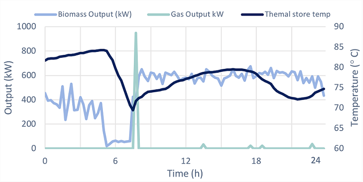
Figure 3: Plant operation over 24h
At other periods the gas boiler is used when the biomass is down, as seen in Figure 4. Across an 8-day period, it's switched on for the day to allow maintenance to the biomass boiler. The monitored data also reveals that there is almost always only one gas boiler being used at any one time. This is clear evidence for the oversizing of the plant at WWHC.
During the periods when only the gas boiler is on, there is a noticeable difference in the performance of the thermal store, which acts more erratically and depletes less. It is also evident from Figure 4 that the thermal store is being underutilised in the system, and possible oversized, as shown between days 5-7 where the thermal store remains at the supply temperature. Nevertheless, the effect of the thermal store on the district heating system is apparent, as seen with the spikes in district heating (DH) power as the thermal store is depleted.
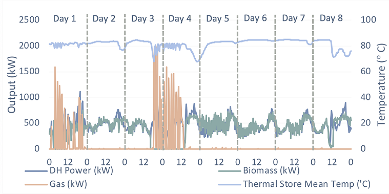
Figure 4: Plant operation over a week
Distribution Layout
The distribution network comprises both buried and building pipework. The buried pipework was determined from a basic layout of the site and Google Earth. The layout is shown in Figure 5 which includes the pipe lengths and the DN specification. The pipework comprises adjacent flow and return pipes with an assumed depth of 0.5m and pipe separation of 0.15m. The internal pipework in the towers is identical on all floors of each tower and this is given in Figure 6. It was not possible to find out the layout in the Terraces for the project. In total there is of 5.6km distribution pipework between the Energy Centre and the dwellings (11.2km including the return pipes). Of this 1.2km is buried and 4.4km distributes the heat within the buildings.
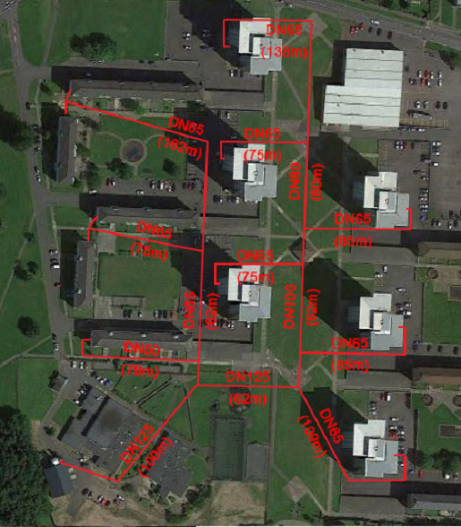 Figure 5: Buried pipework layout |
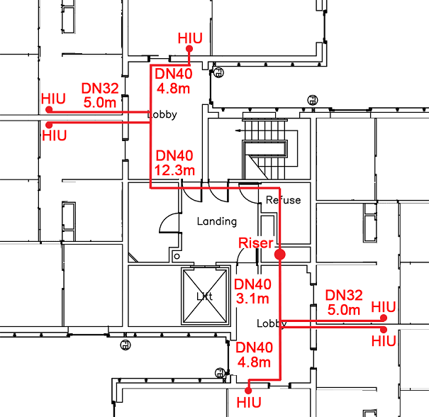 Figure 6: Tower pipework layout |
|---|
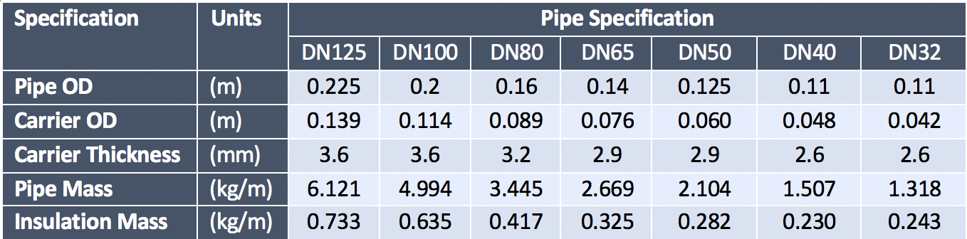
The pipes’ technical specification is provided in Table 2. The carrier pipe was assumed to be P235GH steel (k = 51 W/mK and Cp = 461 J/kgK) while the insulation is rigid polyurethane foam (k = 0.0263 W/mK and Cp = 1450 J/kgK).
Table 2: Distribution Pipe Specifications
Heat Losses
Since its commissioning, the system has suffered from large heat losses during distribution. The meters monitor the heat output from the Energy Centre, the heat arrival at the blocks and the heat consumption of the flats. From these readings, it is possible to determine:
- the total heat input to the network;
- the losses in the buried pipework;
- the losses within the buildings; and
- the heat used by the residents.
This analysis was conducted over 6 months, from July 2016 to December of the same year. This allowed the seasonal variation of the system to be identified. Figure 6 shows the results from this analysis.
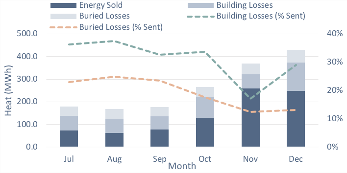
Figure 6: Heat Bought and Losses in the System
The losses are generally larger in winter than in summer months. This is for two reasons: the average temperature difference between the DHS water and the ambient air/ground is larger; and the heating load is larger leading to more heat being in circulation. However, as a percentage of the total heat input to the system each month, the losses in summer are more significant. In summer and autumn, over 50% of the inputted heat is lost before delivery. This is due to the residency time of the heat in the distribution network arising from smaller space heating demands in these months.
Heat loss is more significant within the buildings than in the buried pipework across the year. This had previously been identified and remedial steps have been taken: the insulation around the DN32 pipes (from Figure 6) was replaced to match the design specification. Also losses would be expected to be higher since there is nearly 4 times the length of flow and return pipes for building distribution than buried distribution.