Selection of Software

Once the decision had been taken to focus the project on district heating modelling an investigation was carried out into the various software available, to find a potential tool to model the system. As displayed in Figure 1, the criteria taken into account during this phase can be categorised as follows:

• Accessibility - Availability of the application within the project time constraints and within reasonable cost of licence. As well as the group's previous knowledge and the software's level of difficulty;
• Functionality - Program capabilities to model the heating network with all important plant components and ability for detailed dynamic simulation. As well as the capability for real data from the site to be fed into the model and the level of result data the application can generate.

After this research a list of 6 potential applications was compiled: Excel, Homer Pro, energyPRO, MATLAB, TRNSYS and ESP-r.

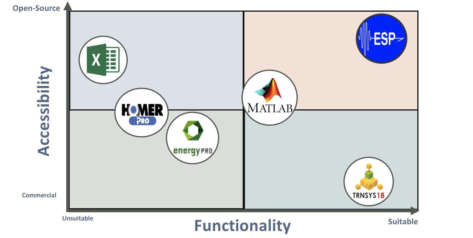
Figure 1: Software Appraisal

On the left side of the graph there are 3 applications which were quickly rejected due to the simulation limitations they entailed. They either couldn’t do the dynamic simulation required or were only capable of high-level modelling. On the right side of the graph are the applications that most closely met the requirements. MATLAB, however, was rejected due to the time required to write the code from scratch, while TRNSYS was eliminated due to the expensive software licence that was required. In the end the optimal choice was ESP-r, a software developed at the Univeristy of Strathclyde, with newly developed plant modules.

Overview of ESP-r

ESP-r (Environmental Systems Performance-Research) is a software created by the University of Strathclyde and was originally developed as a modelling tool for buildings performance simulation. The tool is equipped to model heat, air, moisture, light and electrical power energy flow-paths at user specified boundaries.

ESP-r is based on a finite volume, conservation approach in which a problem specified in terms of geometry, construction, operation, leakage, distribution etc. is transformed into a set of conservation equations which are then integrated at successive time-steps in response to stochastic climate, occupant and control system influences. The simulation timestep can be adjusted between a fraction of a minute to an hour, as required.

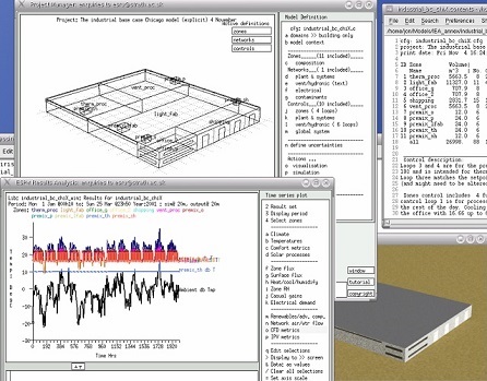
Figure 2: ESP-r

ESP-r has a world-wide development community and is available for free under Open Source licencing. It’s widely used for consultancy, research and teaching. The power behind ESP-r is in its holistic nature and range of features. The weakness of this application, however, can be the fact that specialist features require knowledge of the particular subject due to lack of documentation. As previously mentioned, the program was originally dedicated for building simulations, however, recently added plant modules allows the capability for modelling of district heating networks.

Components and Control

The new ESP-r plant modules allow the modelling of the full district heating system at WWHC to various levels of detail. Each module is discussed in turn below:

Shell Boiler

Heat input to the circuit occurs in a boiler element, in which the combustion process of the fuel and the heat exchange from the combustion chamber to the circulating water are not considered. Heat is added directly to the circulating water. Also, convective heat loss occurs through the boiler casing although this is only indicative, as the true heat loss characteristics are not accurately modelled. The boiler attempts to maintain a setpoint temperature at the outlet using a PID controller.

Load

Heat removal is achieved through a dummy load. As with the boiler the heat exchange of the real plant is not modelled. The dummy load reads a data file column at every simulation time-step and removes heat equating to the corresponding value. A minimum outlet temperature is defined such that heat cannot be removed from the inlet water past the given point – this is recorded as a ‘heat deficit’.

Flow Components: Pump, Diverter and Converger

The water is circulated by a pump. Pressure is not considered in the current modules and is uniform downstream of the pump. The pump module defines a mass flowrate meaning it can change across the component. The mass flow rate is controlled to be inversely proportional to the return water temperature.

The diverter allows the flow to be split into two streams. At every time-step, the fractional amount of flow down each branch is defined. It can either be controlled directly or by another component (i.e. the thermal store). The converger brings together and mixes two flows - no control is applied to it.

Figure 4: Pump	Figure 5: Converger	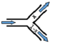Figure 6: Diverter

Pipework

Heat is lost from the above-ground pipework according to the pipe’s overall heat transfer coefficient. The containment temperature can be defined or taken from the ambient air. Pipework could also be associated with a ESP-r thermal zone: integrating the plant and building models.

The main distribution pipework in the network comprises an insulated flow and return pipe, buried in a common trench. Heat transfer from the pipes is not all lost to the surroundings but a portion is transferred from the flow to the return pipe through the ground. The module simulates transient heat loss using the theory and equations outlined by Bohm (Bohm, 2000). In the model the buried pipework must be carefully linked to simulate the real thermal interactions.

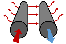
Figure 7: Heat transfer in buried pipes.

Thermal Store

The thermal store is represented as a stratified tank (with a temperature gradient through it). It serves two purposes:

• The storage of heat to offset supply and demand temporally; and,
• The balancing of the flow on both halves of the circuit.

The direction of flow through the store depends on the difference in the circuit flow rates. An example of charging and discharging in the model are represented in Figures 8 & 9, respectively. The store currently acts in a passive way and is not actively controlled.

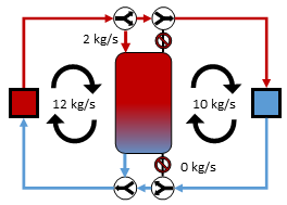Figure 8: Charging of thermal store	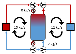Figure 9: Discharging of thermal store

ESP-r District Heating Model

Using the new plant components it is possible to construct a dynamic, thermal model of the WWHC system. Yet a significant question still exists in regard to the level of detail of an initial model of the system. It would be possible to model each flat as an individual load and to model the interconnecting pipework, however, this would lead to a model with ~550 loads and 1000's of distribution pipes. The time limits of the project (and potentially the computational power of ESP-r) would not allow this.

In place, it was decided to model each of the buildings as a single load and to investigate individual flats at a later date (time permitting). The non-domestic loads were omitted because no data or occupancy behaviour were known for these loads. The terraces, similarly, did not have available data and so for simplicity these were also modelled as a single load. The model allows the overall operation of the system (and the new ESP-r modules) to be analysed. This final model is shown schematically in Figure 10.

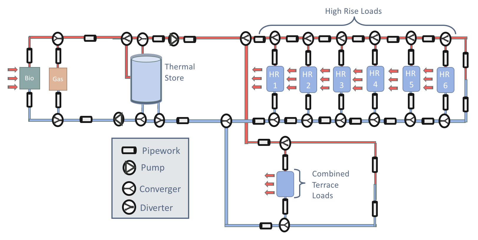
Figure 10: Schematic of ESP-r DH Model

As indicated above, the circuit can be thought of as two half circuits balanced by the thermal store. The mass flow rate in both halves and the flow rate in each load branch are controlled in an attempt to maintain sufficient heat circulation in all parts of the circuit. This means that if the control temperature begins to drop the mass flowrate increases in a linear manner which increases the amount of available heat and vice versa.

The simulations were run over single months at minute time-steps. Long periods could be run, however setting the control parameters in such a way that the loads were met over different seasons was complex. Adaptive control logic (changing it based on the time or sensed conditions) could overcome this. Increasing the time-step introduced numerical instability during solution, which led to long simulation times.

Resident Demand

The heat demand on the system is the principle input to the model, where the demand profiles required depend on the simulations to be run and the questions asked. The Smart Meters in the dwellings of West Whitlawburn log the energy use in the property, which allowed real demand profiles to be used in the model. The demand of 49 flats in Arran Tower was available from March 2016 to Feburary 2017 inclusive. These were investigated both individually and in an aggregate way.

User Types

The usage characteristics vary considerably from flat to flat. This may be due to the location of the flat within the block or due to the economic situation of the residents. The total monthly heat usage between flats is far more considerable than the variation of an individual flats use from month to month. Figures 11 and 12, present the total monthly consumption of each flat over summer and winter months.

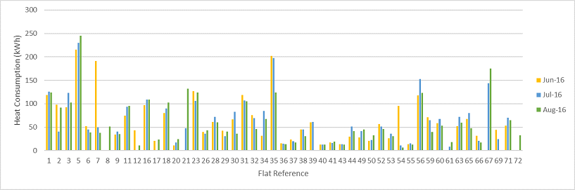
Figure 11: Flat demands over summer months

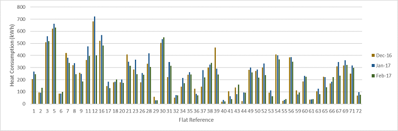
Figure 12: Flat demands over winter months

The data revealed that many residents are consistently low users (i.e. 40, 55, 61 and 72) and others are consistently high users (3, 5 and 56). Many others exhibit low use in summer and high winter use (12, 30 and 54), however, the variations across the three months in each season are generally small. The demand profiles from individual flats also indicate highly variable user behaviour between different dwellings. Approximately 20% of the demand profiles had consistent low usage (as shown in Figure 13). Heat was used predominantly in the mornings and so it was assumed that this was hot water used for showering. A further 20% featured high and erratic usage (i.e. Figure 14), which could be due to higher levels of occupancy and larger households. The vast majority of other properties displayed highly variable behaviour that could not be easily categorised.

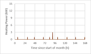Figure 13: Consistent Low Use	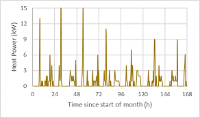Figure 14: Erratic High Use

The flat demands highlighted:

• Highly variable behaviour between tenants;
• A significant proportion of low users; and,
• The difficulty in categorising and grouping user types.

For this, and other reasons, it was decided that for the purposes of this project full blocks would be considered as single loads.

Block Demand Profiles

For the model, it was necessary to create separate aggregate demand profiles for each block. A method was used to transform the aggregate demand profiles from separate months into a single month. Space heating demand is principally influenced by the ambient dry bulb temperature. Therefore, to transform the demand profile from one month to the other, the relative heating requirements due to the ambient air temperature were taken into consideration.

Using hourly climate data collected in Glasgow over the same period, the heating degree hours were calculated for every time step. From these a weighting factor profile was constructed which related the ambient air temperature between the same time in two different months. The demand data was multiplied by this factor to convert the demand into the desired month. An example of this is provided in Figures 15 and 16, where the demand profile from October is transformed into a profile representative of November.

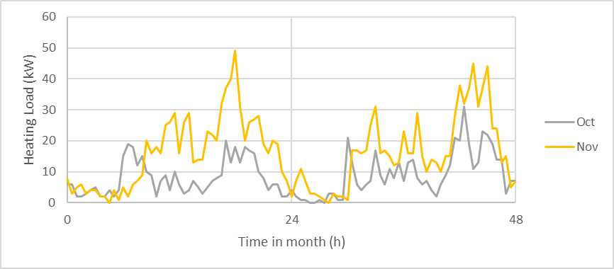Figure 15: October Demand	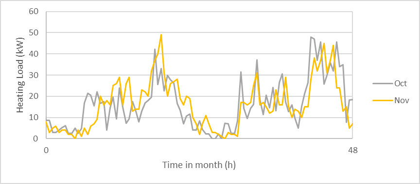Figure 16: Modified to November Temperatures

Although this method represents a simple and approximate approach, the resulting demand profiles were improvements on the original profiles. In this way, six months of data could be transformed into demand profiles for six towers over one month. An issue existed with the method in summer months when the heating degree days are low and most of the heat demand is for domestic hot water which generally doesn't vary with air temperature. For these months random number generaters were used to augment the method used here.