Supply

In order to find the potential energy generation of a certain land area, the specific energy density must be calculated. A spreadsheet tool was developed for both wind farm and solar array generation.

Solar Energy

In order to calculate the output power (Watts) of a single solar panel, the angle of incidence of the sun on the solar panel must be found. This changes with time and the solar PV spreadsheet model in this case calculated output power in hourly increments. The weather data taken from ESRU was entered into the model so that various solar positioning angles could be found.

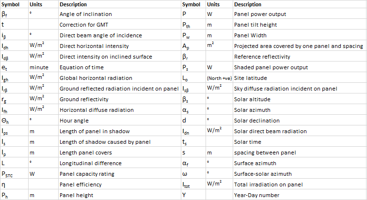
*All the nomenclature for the following equations can be seen in Table 1

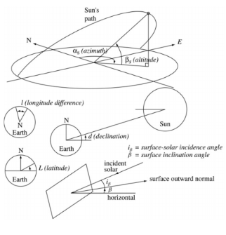
First, the solar declination and equation of time can be found depending on the time and day of the year.

d = 23.45 sin(280.1 + 0.9863Y)

where Y = Day of the year, (eg Jan 1 = 1 & Dec 31 = 365)

e_t= 9.87 sin(1.978Y - 160.22) - 7.53 cos(0.989Y - 80.11) - 1.5 sin(0.989Y - 80.11)

Depending on the users entered longitude, the local solar time can be calculated

S_t= (L_o/15) + (e_t/60) + t

The hour angle can then be calculated as a function of local solar time

h = 15 (12 - S_t)

From these functions of time the solar elevation, the relative height of the sun, can be found.

b_s= sin ^-1(cos L cos d cos h + sin L sin d)

The solar azimuth angle can be obtained by,

a_s = sin ^-1((cos d sin h) /cos b_s)

Finally, the solar incidence angle can be calculated.

i_b = cos ^-1((sin(b_s)) cos(b_f) + cos(b_s) cos(w ) sin(b_f))

The angle of incidence is the direction component of the direct solar on the panel, therefore combined with the magnitude of direct normal solar, the direct solar on panel can be calculated.

I_db = I_dn cos (i_b)

There are two other parts that contribution to the total solar radiation on a panel, these are the ground reflected and diffuse radiation.

I_rb = 0.5 (1 - cos (b_f)) (I_dh + I_fh)r_g

I_sb = I_fh {0.5 [1 + cos (b_f)]}.{1 + [1 - (I_fh² / I_gh²)] sin³0.5b_f} {1 + [1 - (I_fh² / I_gh²)] cos² I_b sin³ (b_s)}

The total solar irradiation on the panel is the sum on the three components.

I_tot = I_sb + I_rb + I_db

The panels average hourly electrical power output can then be calculated depending on its capacity rating, reference reflectivity, efficiency rating and ambient temperature.

P = P_stc (I_tot /1000)(1 - b_r(T - 25)) h

The hourly output values of a single solar panel are then integrated over the year to find the yearly energy output and capacity factor. The number of solar panels that can be placed in a certain area of land is calculated depending on the panel height and inclination, spacing between panels and area of land. Assuming there are no gaps between the panels horizontally, the space a single panel covers can be found.

A_p = P_w ((P_h cos (b_f)) + s)

Knowing the area each panel requires, the number of panels that can fit over a certain land area can then be calculated.

No. Panels = 0.9777(Available Land / A_p)

*0.997 is a constant that was calculated using Helioscope, required to rectify the number of panels because of differences in shapes of areas of land.

---

Shading

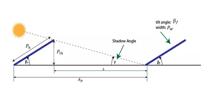
The above values would be enough to give a rough value of the output of a solar array depending on its area. However, to generate a more accurate output that changes depending on how much of the panel is in shade from the panel in front, more calculations must be made.

First the length of shadow generated by a solar panel must be found.

l_s = P_th / tan (b_s)

Then, the length of shadow on the solar panel behind can be calculated.

l_ps = sin(b_s)(l_s - s) / (sin (180 - b_f - b_s)))

From this, the percentage of panel in shadow can be calculated.

% = l_ps / P_h

Therefore the output power panel including shading calculations can be found.

P_s = (1 - %) x P

These values can be integrated over the course of year to find the yearly energy output of a single solar panel including shading. Multiplying by the number of panels in an array; the total array output including shading can be found. The total array energy output divided by the area of land, therefore, gives the energy density.

Single Panel Validation

The model was validated for a single solar panel without the shading. Panel and location data were entered into renewables.ninja and adding a 10% drop in efficiency for a single panel to account for a decrease in power output over time. The model was hence validated because there was a 9% difference in capacity factor, deemed within an acceptable range.

Helioscope Validation

In order to validate the shading calculations, Helioscope, a professional solar array software package was used (Helioscope.com, 2019). The same area, location, weather and panel data were inputted in the solar calculation tool and Helioscope software. The monthly energy output values are compared in Figure 3.

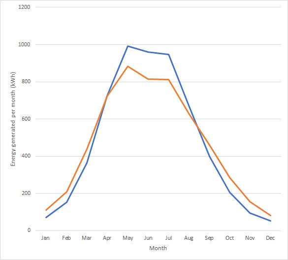
Whilst the two models show variations in monthly output, the difference between the yearly results is only 1%, well within the acceptable margin for error.

Calculating Optimum Angle of a Single Solar Panel

The optimum angle of inclination for a single solar panel can be calculated by changing the angle and to find the largest yearly energy yield without the solar shading calculations. This was found to be 30° to the horizontal.

Calculating best angle for array

Optimising for the largest energy yield over a certain land area requires shading calculations. The following graph was generated using the solar calculation tool and shows how the energy density changes with spacing between the panels and angle of inclination.

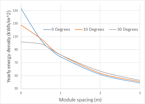
At a 1m spacing between the panels to account for space for technician maintenance, the energy output of an array is around the same for a 10° & 30° inclination, however, the 10° inclination generates less panels over the land area. This makes the 10° inclination preferable because it reduces cost and was therefore selected as the best configuration for Glasgow.

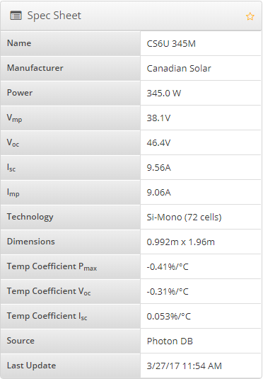
The type of solar panel used for these calculations is a CS6U 345M panel, the specifications of which can be seen in Figure 6.

Energy Density

The final value calculated for the energy density of a solar array in Glasgow is 82 kWh/m² +/- 10% to account for yearly weather variations

---

Wind Resource Analysis

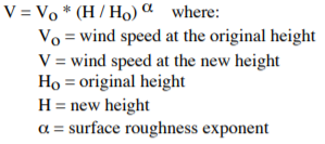
In order to calculate the total energy output of the turbine, it is required to analyse actual wind data from the chosen location, Glasgow in this case. By taking hourly wind speeds, they can be converted from baseline height conditions (10 metres) to the hub height of any of the pre-existing wind turbines (1 kW, 5 kW, 10 kW, 50 kW) by using the Gipe power law (Equation 19), and appropriate surface roughness (Chandler et al).

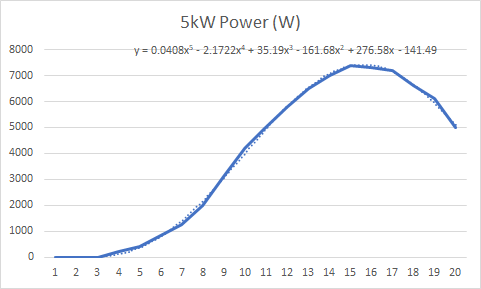
To generate a power curve within the decision support tool, a graph was created using the relevant data for wind speed and corresponding power generated. From this, the equation of the line was found by generating a line of best fit, using a higher order quadratic equation in order to ensure a higher degree of accuracy (Figure 7). This equation could then be used to obtain wind turbine power from the already known wind speeds. The cut in and cut out wind speeds were used to eliminate any power results above or below the maximum and minimum respectively.

The method used accounts for the surface roughness of the land in the run up to the turbine, however does not account for turbulence induced by buildings. Accounting for this would require an individual cite appraisal at each site where wind turbines were proposed, and would depend on the turbines proximity to buildings, height of surrounding buildings, and the extent to which the buildings extended in the direction of the prevailing wind.

Inter-model validation was used to ensure the results were correct. Inter-model validation was used as complete data-sets containing weather data, power generation, and power curves for the wind turbine were not readily available. For this purpose, HOMER (Homerenergy.com, (2019)) and Renewables.ninja (Renewables.ninja, (2019)) were used.

Wind turbine spacing is important to ensure the turbulent flow of air from the turbine in front does not adversely affect the turbine behind more than can be helped. Recommendations for turbine spacing vary, with most current wind farms using a spacing of between 5 and 10 rotor diameters depending on the layout, although up to 15 can also be used (Phys.org, 2019). Due to the space limitations of vacant and derelict land, a smaller spacing of 7 rotor diameters was used however the optimum layout would depend on the site in question. Factors such as surrounding topography and prevailing wind direction play a key role in deciding optimum layout. The number of turbines that can be fitted to an area is then found by the following equation:

Number of turbines=((ÖAvailable land)/d_r)²

*where d_r is wind turbine rotor diameter

---

References

1. Anon., n.d Chile renovables [Online]
   Available at http://www.chilerenovables.cl/[Accessed 6 Apr. 2019].
2. Helioscope.com. (2019). HelioScope: Advanced Solar Design Software. [online]
   Available at: https://www.helioscope.com/ [Accessed 6 Apr. 2019].
3. Greenrhinoenergy.com. (2019). Solar Photovoltaics | Impact of shading. [online]
   Available at: http://www.greenrhinoenergy.com/solar/performance/shading.php[Accessed 6 Apr. 2019].
4. Homerenergy.com. (2019). HOMER - Hybrid Renewable and Distributed Generation System Design Software. [online]
   Available at: https://www.homerenergy.com/ [Accessed 6 May 2019].
5. Renewables.ninja. (2019). Renewables.ninja. [online]
   Available at: https://www.renewables.ninja/ [Accessed 6 May 2019].
6. Phys.org. (2019). Study yields better turbine spacing for large wind farms (w/ Video). [online]
   Available at: https://phys.org/news/2011-01-yields-turbine-spacing-large-farms.html [Accessed 7 May 2019].