Structural Analysis
Introduction
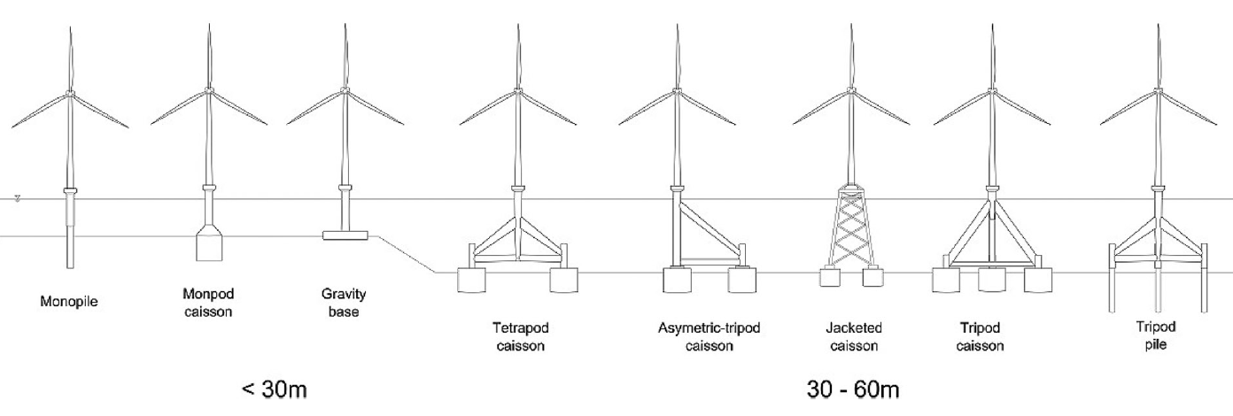
Monopiles have been used as a foundation for numerous offshore wind farms. They are one of the most inexpensive solutions for supporting structure of offshore wind turbines (OWTs). The price of a foundation is an important factor, as it can mean over 30% of overall costs. This may highly affect the financial feasibility of a project. However, the usage of relatively low-priced monopiles is limited due to the sea depth and a type of seabed at the site.
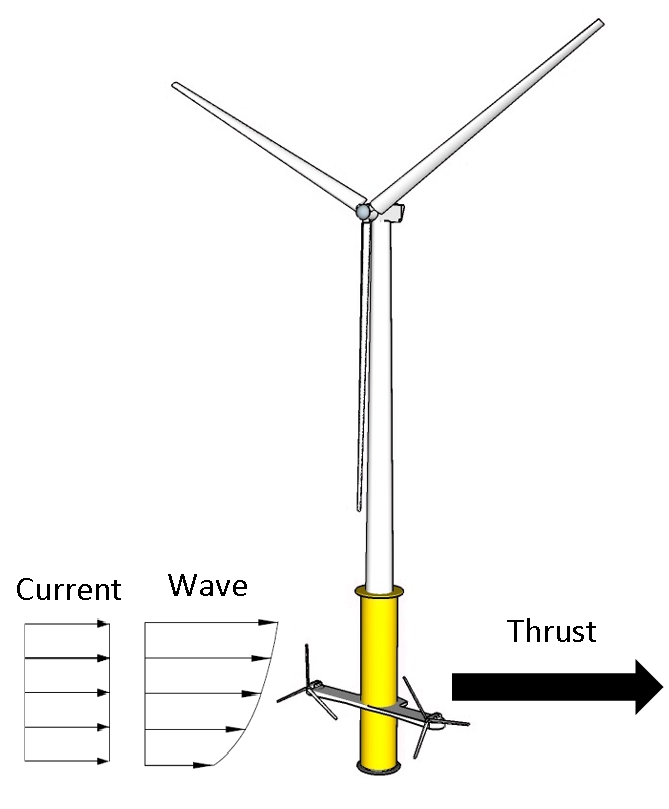
As the highest tidal resources are in locations of limited sea depth, we decided to use monopile as a foundation for our Hybrid Offshore Wind and Tidal device (HOWaT).
One of the objectives of our project was to investigate the influence of attaching a tidal turbine to the supporting structure. The effects of an extra load applied have been assessed based on a comparison of an OWT and a HOWaT device. This allowed determining the additional costs of a HOWaT's monopile. Moreover, simplified natural frequency calculations were carried out to examine the possibility of high vibration.
Structure and turbines description
As described in Wind Concept, for the purpose of this project we have decided to use 5-MW Reference Offshore Wind Turbine developed by National Renewable Energy Laboratory (NREL). The dimensions and properties of the wind turbine, tower and a monopile were adopted based on Offshore Code Comparison Collaboration (OC3) Phase II [2] and [3].
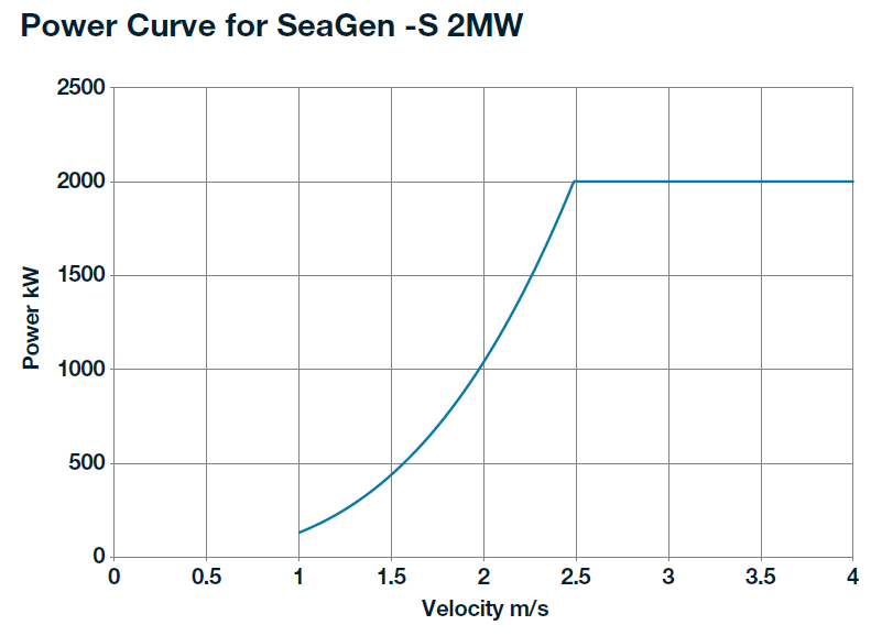
Tidal current turbine parameters were based on SeaGen S 2MW- developed by Marine Current Turbines [4].
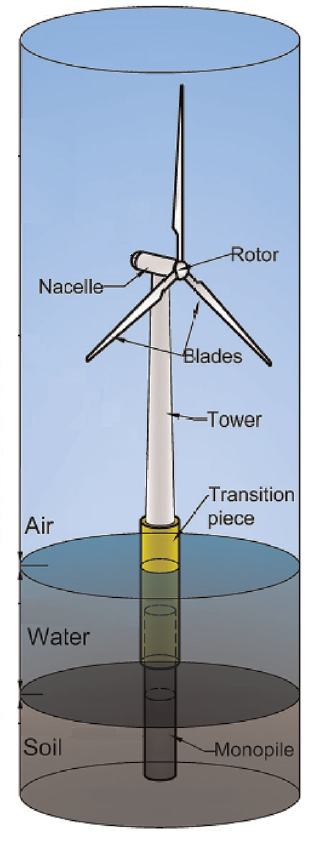
The constant monopile outer diameter (Φ6000 mm), the same as in [3], and the constant thickness of the monopile of 70 mm were used. Transition piece was skipped in the model, however, its mass was taken into account. Thus, the monopile extends from the mud line to the tower baseline.
The tower is the same as the one used in Phase II of [3]. Its base and top are located 10m and 90m above mean sea level (MSL) respectively. The tower thickness and diameter were modelled as linearly tapered from base to the top, where outer diameter and thickness at the baseline and the top are Φ6000 x 27 mm and Φ3870 x 19 mm respectively. Both the monopile and the tower were assumed to be made of steel.
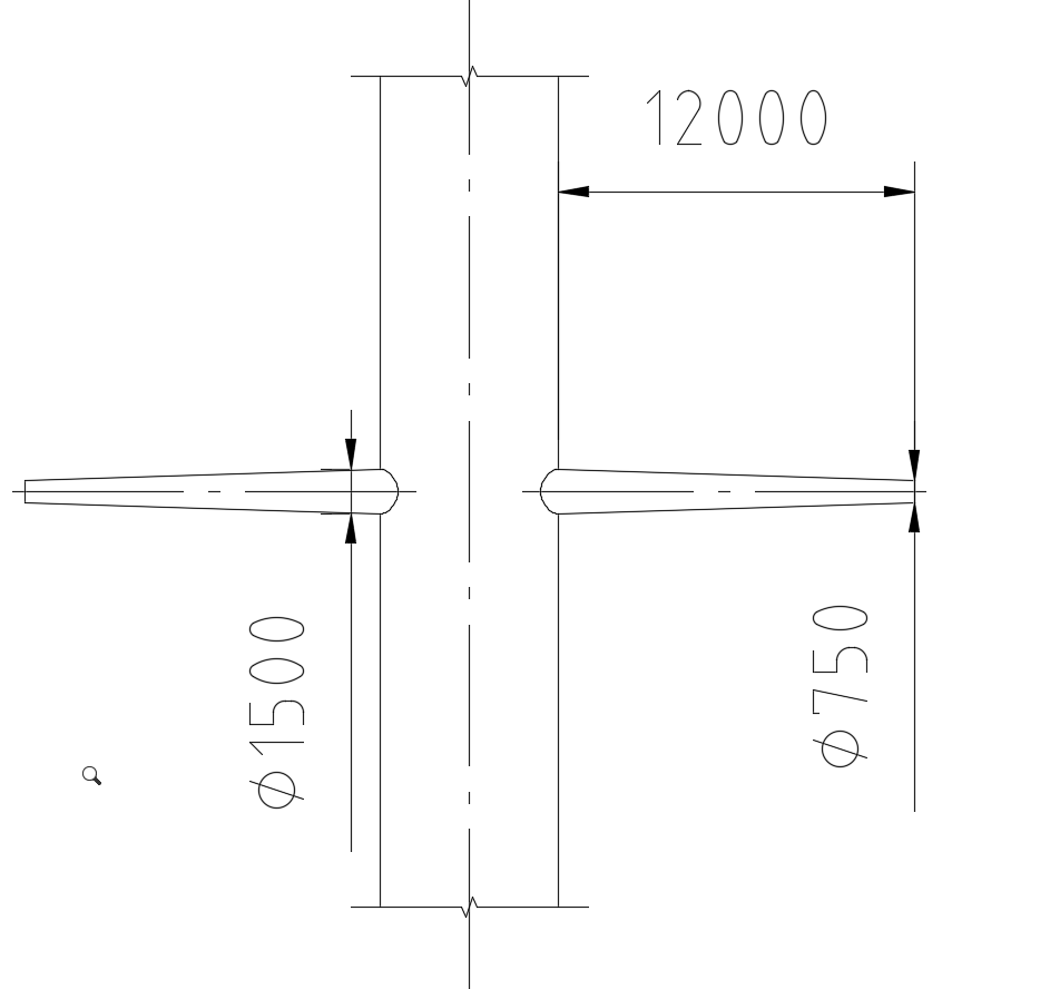
The additional supporting structure of tidal turbine has not been modelled, as it was not in the scope of our project to investigate its stresses. Since the tidal turbines are assumed to work simultaneously, no torsional loads are expected. The loads caused by the tidal turbine can be applied directly to the monopile. Nonetheless, a simplified supporting structure was used to determine its weight and the current drag on the structure - a tapered pipe with the thickness linearly tapered from the monopile (30 mm) to the tip (15 mm). The dimension can be found in Figure 3
Methodology
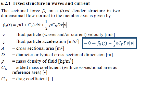
The main purpose of the structural analysis was to determine and compare stresses in the foundation of an offshore wind turbine (OWT) and a hybrid wind & tidal device (HOWaT). To make comparison easy, Von Mises stresses were chosen to be calculated and analised. Von Mises stress, also known as equivalent stress, is widely used in engineering to verify whether the structure will withstand a load condition.
As the structure was described, the next step was to determine the loads acting on it. Since the monopile is embedded in the seabed, that has to be taken into account and soil-monopile interaction was modelled as well. Additionally, the natural frequency of the structure was calculated to determine if it is within a safe frequency range.
Loads
There are different kinds of loads acting on OWT and HOWaT. Some standards have been issued by institutions such as DNV GL [5] and British Standards Institution [6] and these loads and the methods to calculate them are listed there. BS EN 61400-3:2009 [6] specifies following loads.
- Gravitational and inertial loads - static and dynamic loads due to gravity, vibration, rotation and seismic activity
- Aerodynamic loads - static and dynamic loads caused by the airflow
- Actuation loads - results from the operation and control of the wind turbine
- Hydrodynamic loads - dynamic loads caused by the water flow
- Sea ice loads - static load due to temperature fluctuations or changes in water levels and dynamic load caused by motion of ice floes
- Other loads
For simplicity of our project, some of the loads were omitted. We have taken into account only dead load, aerodynamic and hydrodynamic loads, as those have the highest impact on the structure. Moreover, the scope of this project is comparing HOWaT and OWT rather than the verification of a particular construction. The environmental conditions used to obtain the external forces were based on a case study location - Isle of Islay. The calculations details of each kind of load is presented below
Dead Load
The dead load for both OWT and HOWaT is the sum of the weight of the components:
- Wind turbine - rotor, hub, nacelle
- Tower
- Transition piece
- Monopile
- Tidal Turbines
- Tidal turbine supporting structures
The mass of the wind turbine components has been taken from [2] and [3]. The mass of the tidal turbines was assumed to be equal to the power trains weight as specified in SeaGen Brochure [4].
The mass of the tower and monopile has been calculated by Finite Element Analysis (FEA) software based on the volume of modelled material and it was automatically considered in the calculations. The assumed effective density of steel for both components is 8500 kg/m3. This value is higher than a typical value in order to account for bolts, paint, welds, and flanges not considered in thickness data [3]. It can also be justified as considering the weight of gross thickness, while for the purpose of structural analysis the net thickness is used to include effects of corrosion during the lifetime of the structure. This was not considered within the scope of our project.
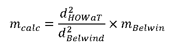
Due to the lack of detailed guidance to estimate transition piece weight, the adjusted value of the existing wind farm transition piece was calculated. It was assumed that the weight of the transition piece is proportional to the squared monopile diameter. The mass of Belwind project [6] transition piece was 120 tonnes, whereas the monopile diameter was 5 m.
As mentioned above, the tidal turbine supporting structures were simplified. The volume of tapered pipe (dimensions) was calculated assuming that thickness was linearly tapered from the monopile (30mm) to the tip (15mm).
The mass of non-distributed components is included in Table 1.
| Component | Mass [kg] | Position above MSL [m] |
|---|---|---|
| Wind | ||
| Rotor | 110 000 | 90 |
| Hub | 56 780 | 90 |
| Nacelle | 240 000 | 90 |
| Structure | ||
| Transition piece | 172 800 | 0 |
| Tidal | ||
| Turbine | 60 000 | -14 |
| Supporting structure | 17 798 | -14 |
Aerodynamic Loads
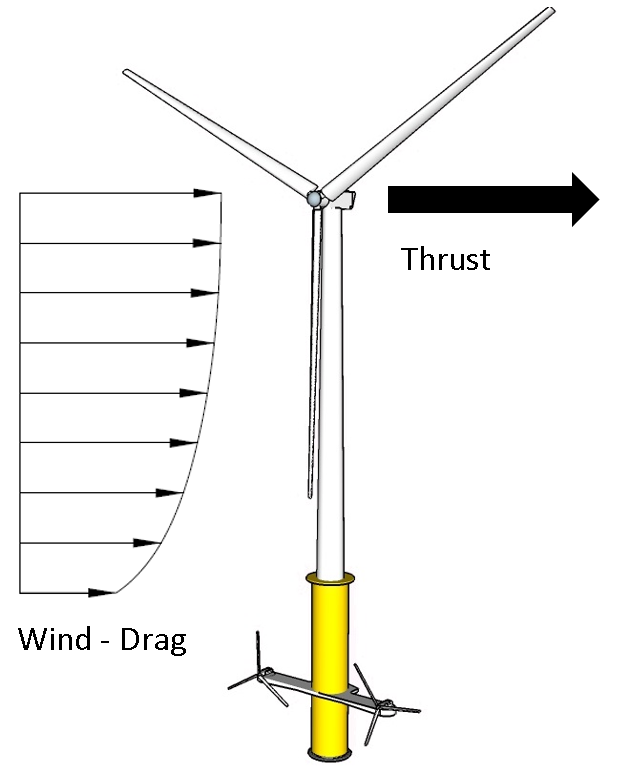
Flowing air acts on the structure and it causes aerodynamic loads. The load on a static structure is wind drag, whereas the load on rotating elements is thrust. The whole structure above MSL is subject to the drag. The thrust acts only on a rotor, however, it has a substantial influence on bending moment within the foundation as it is applied to the tower on the top of it.
Thrust
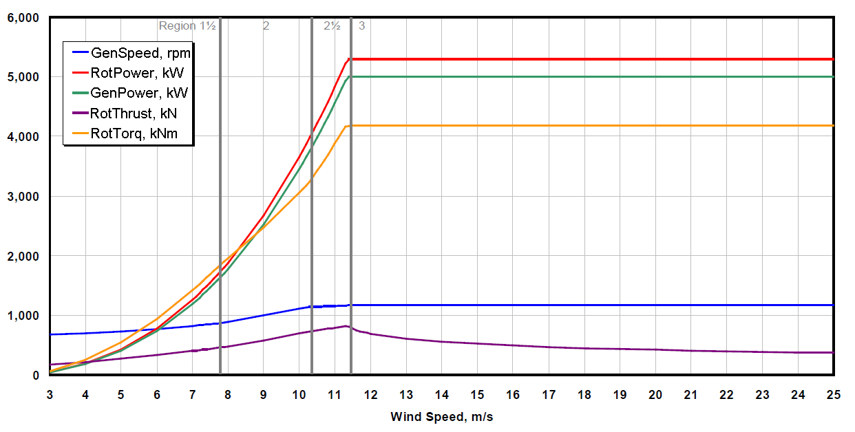
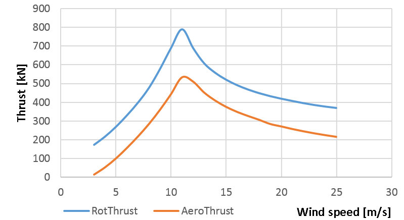
The characteristics of NREL 5MW turbine include the rotor thrust curve (see RotThrust in Figure 6). However, an aerodynamic thrust (AeroThrust) curve has been also calculated based on the power curve data (see RotPower in Figure 6). As we assumed the method of calculation of thrust is the same for water and air, it is described in hydrodynamic thrust section. The calculated values are significantly different.
It can be justified by the fact that Rot Thrust is not an aerodynamic thrust. Along with the thrust, it takes into account inertia and gravity of the rotor as well. Figure 7 shows the comparison of both curves. For further analysis, the higher value was taken.
FRotThrust = 790.6 kN
FAeroThrust = 532.5 kN
Drag
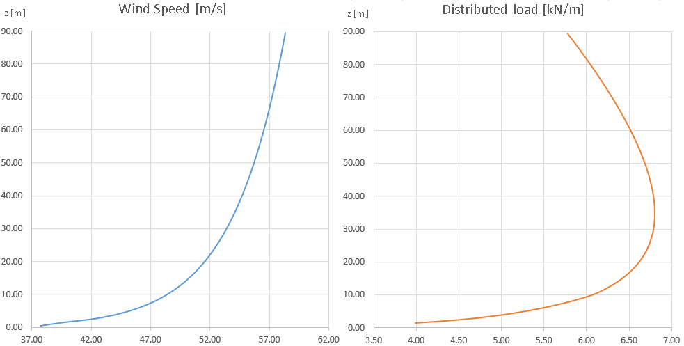
The Wind drag on the tower was calculated according to BS-EN 1991-1-4:2005+A1 procedure [8]. The basic wind velocity was obtained from the National Annex [9] to the code. The velocity was then corrected based on the procedure, as explained in Figure 9 and mean wind velocity was obtained.
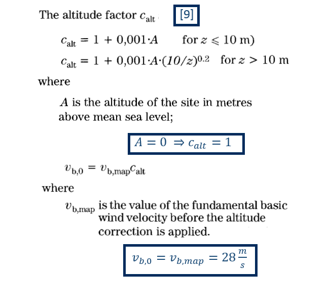
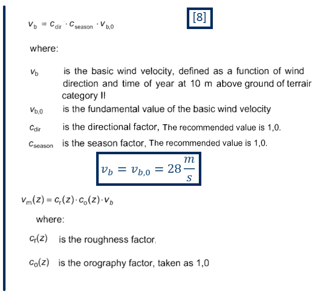
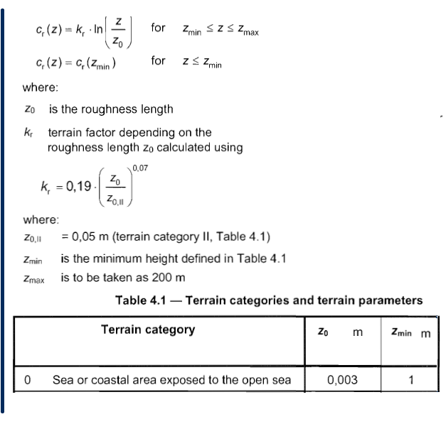
The mean wind velocity does not take into account wind gusts. Moreover, turbulence should also be accounted for. Therefore, the further correction was applied and peak velocity pressure obtained. Further details of obtaining wind force according to the procedure can be found in Figure 10.

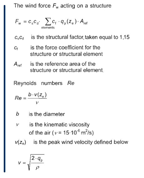
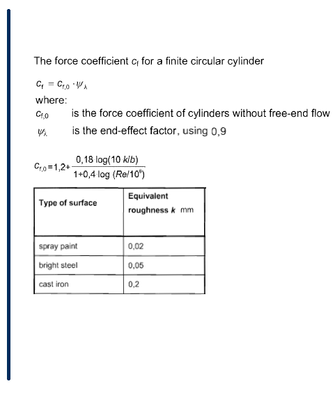
Table 2 shows the simplified summary of calculated values (the height step, 10 m as seen in the table, was different for structural calculations: a step of 1 m was used). Figure 11 illustrates the distribution of peak wind velocity and wind force acting on the structure.
| h [m] | b [m] | z [m] | cr [-] | vm [m/s] | lv [-] | qp [Pa] | v [m/s] | Re [-] | cf,0 [-] | cf [-] | cscd [-] | A [m2] | Fw [N] |
|---|---|---|---|---|---|---|---|---|---|---|---|---|---|
| 0 | 6.00 | 5 | 1.16 | 32.40 | 0.135 | 1276 | 45.20 | 1.81 × 10⁷ | 0.776 | 0.699 | 1.15 | 60.0 | 61 533 |
| 10 | 6.00 | 15 | 1.33 | 37.20 | 0.117 | 1576 | 50.20 | 2.01 × 10⁷ | 0.781 | 0.702 | 58.7 | 74 729 | |
| 20 | 5.73 | 25 | 1.41 | 39.40 | 0.111 | 1726 | 52.60 | 2.01 × 10⁷ | 0.782 | 0.704 | 56.0 | 78 290 | |
| 30 | 5.47 | 35 | 1.46 | 40.90 | 0.107 | 1828 | 54.10 | 1.97 × 10⁷ | 0.784 | 0.705 | 53.3 | 79 095 | |
| 40 | 5.20 | 45 | 1.50 | 42.00 | 0.104 | 1906 | 55.20 | 1.91 × 10⁷ | 0.785 | 0.706 | 50.7 | 78 443 | |
| 50 | 4.94 | 55 | 1.53 | 42.90 | 0.102 | 1969 | 56.10 | 1.85 × 10⁷ | 0.785 | 0.707 | 48.0 | 76 866 | |
| 60 | 4.67 | 65 | 1.56 | 43.60 | 0.100 | 2022 | 56.90 | 1.78 × 10⁷ | 0.786 | 0.707 | 45.4 | 74 638 | |
| 70 | 4.40 | 75 | 1.58 | 44.20 | 0.099 | 2069 | 57.50 | 1.69 × 10⁷ | 0.787 | 0.708 | 42.7 | 71 921 | |
| 80 | 4.14 | 85 | 1.60 | 44.80 | 0.098 | 2109 | 58.10 | 1.60 × 10⁷ | 0.787 | 0.708 | 40.0 | 68 819 | |
| 90 | 3.87 | ||||||||||||
Hydrodynamic Load
The motion of sea water causes hydrodynamic loads. The load on a static structure is due to current (it is assumed that it has constant velocity) and wave drag, whereas the load on rotating elements of a tidal turbine is thrust. The structure below MSL is subject to the hydrodynamic load.
Thrust
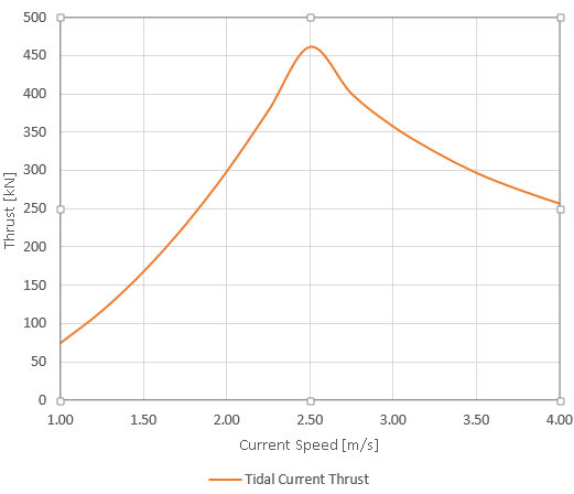
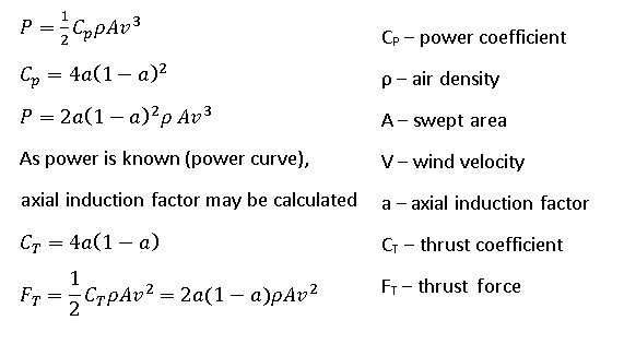
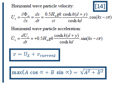
The thrust acts only on a rotor. Although the tidal current velocity and rotor swept area are considerably smaller than that of wind and wind rotor, the magnitude of thrust on tidal turbines is higher. That is because of a significantly higher density of sea water than air density (1025 kg/m3 and 1.25 kg/m3). The method of calculation of both wind and tidal thrust is the same and it is presented in Figure 13 The tidal turbine power curve is shown in Figure 12 and the thrust curve of the tidal turbine (each one) is presented in Figure 14.
In contrast to wind thrust, for tidal thrust, only hydrodynamic thrust was used in the structural analysis. The detailed data for tidal turbine were not available. Furthermore, gravitational and inertial effects on tidal rotors should be significantly lower than those of wind rotor, as they are lighter and smaller. Given that, it was decided to neglect it. Final value applied to the further analysis takes into account two turbines.
FTidalThrust = 922.0 kN
Drag
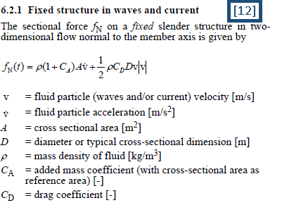
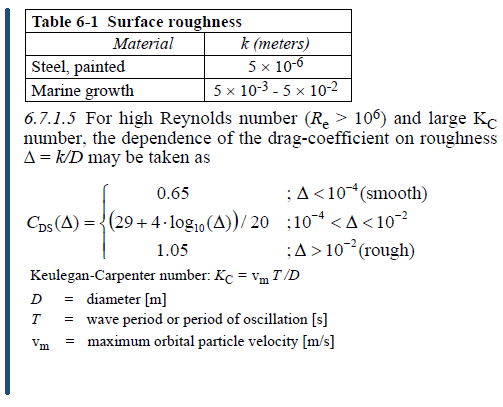
The hydrodynamic drag on the tower was calculated based DNV-RP-C205 [12]. It was assumed that tidal current and wave act on the monopile only. For tidal supporting structures, only tidal current has been taken into account.
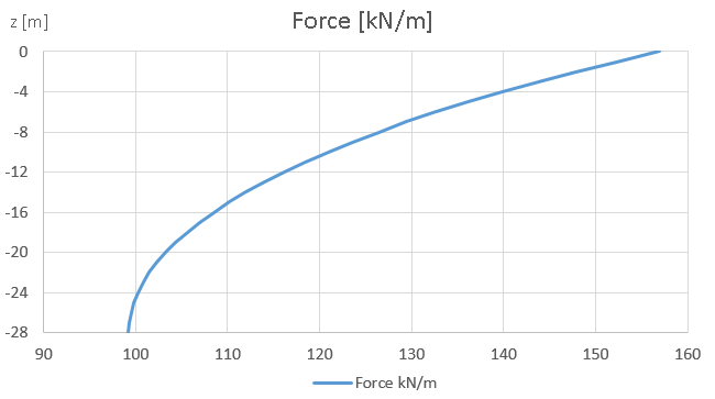
The tidal current profile was assumed to be constant, independent of the position below MSL. As for the location the peak spring tidal current is 3.05 m/s, that value was used in the further analysis. The sea surge has been neglected. Figure 16 shows the hydrodynamic drag calculations (for monopile). Table 4 shows assumed values used to calculate drag coefficient. Added mass coefficient of 1.0 was used.
| No. | 1 | 2 | 3 | 4 | 5 | 6 | 7 | 8 | 9 | 10 |
|---|---|---|---|---|---|---|---|---|---|---|
| T [s] | 3.5 | 4.5 | 5.5 | 6.5 | 7.5 | 8.5 | 9.5 | 10.5 | 11.5 | 12.5 |
| H [m] | 1.5 | 3 | 3 | 4.5 | 5 | 6.5 | 7 | 8 | 9 | 9 |
The drag force was calculated for various wave characteristics. The periods and wave heights were taken for grid point 15609 on Hebrides Shelf from [13]. Maximal wave height values were taken for each wave period. Table 3 shows the parameters of the all the 10 waves investigated.
For each wave, based on calculated drag force, the bending moment value acting on foundation, if fixed at mud line, was calculated. The wave with the highest value of torque was used for the further analysis (no. 9). The distributed drag load acting on monopile is presented in Figure 17.
| Component | Value |
|---|---|
| ν | 1.83 × 10⁻⁶ [12] |
| vcurrent | 3.05 m/s |
| k | 0.05 m |
| Δ | 0.0083 |
| CD | 1.05 |
| CA | 1.0 |
For simplification, drag acting on tidal supporting structures was calculated without considering action of waves. The calculations were conducted in a way similar to that of monopoile. However, inertia and acceleration forces were neglected (Figure 18 shows the minor change applied). The same drag coefficient was used. For structural analysis, a point load equivalent was used. Table 5 presents the summary of drag on supporting structures (each one), where x is a horizontal distance from the tip of the structure towards the monopile. As there are two structures, total load acting on both was applied for the further analysis.
FSuppStrDrag = 130.8 kN
| x [m] | D [m] | v [m/s] | Re [-] | CD [-] | A [m2] | F [N] |
|---|---|---|---|---|---|---|
| 0.0 | 0.750 | 3.05 | 1.23 × 10⁶ | 1.05 | 0.945 | 4577 |
| 1.2 | 0.825 | 1.352 × 10⁶ | 1.035 | 5013 | ||
| 2.4 | 0.900 | 1.475 × 10⁶ | 1.125 | 5449 | ||
| 3.6 | 0.975 | 1.598 × 10⁶ | 1.215 | 5884 | ||
| 4.8 | 1.050 | 1.721 × 10⁶ | 1.305 | 6320 | ||
| 6.0 | 1.125 | 1.844 × 10⁶ | 1.395 | 6756 | ||
| 7.2 | 1.200 | 1.967 × 10⁶ | 1.485 | 7192 | ||
| 8.4 | 1.275 | 2.090 × 10⁶ | 1.575 | 7628 | ||
| 9.6 | 1.350 | 2.213 × 10⁶ | 1.665 | 8064 | ||
| 10.8 | 1.425 | 2.336 × 10⁶ | 1.755 | 8500 | ||
| 12.0 | 1.500 | |||||
| TOTAL | 65383 | |||||
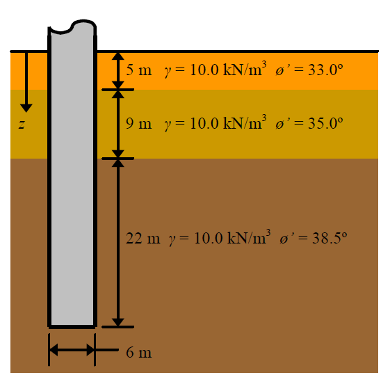
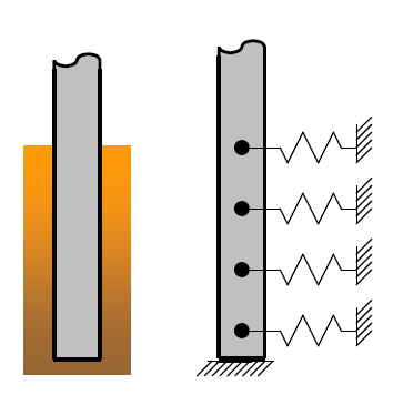
Soil-monopile interaction
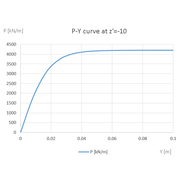
A similar approach to the one presented in Phase II of OC3 [3] was used to model pile-soil interaction. The monopile foundation uses lateral loading due to soil interaction to withstand the loads induced in the HOWaT structure. We have decided to use the same length of monopile embedment. An assumption was made that in our location the seabed consists of sand. We have used 3 layers to represent the soil profile. As distributed springs model was decided to be used, P-Y curves for various positions were obtained according to Recommended Practice of American Petroleum Institute (API) [15]. These values were slightly different than those used in OC3 project [16], especially for lower positions. This was caused by the fact that we have not corrected the depth to reflect the layered soil, while the OC3 values were based on equivalent depths. Thus, we decided to use the values calculated in OC3. Figure 19 and Figure 20 illustrate the details of soil-pile interaction model, whereas Figure 21 shows an example of P-Y curve used in the structural analysis.
Vibrations - Natural Frequency
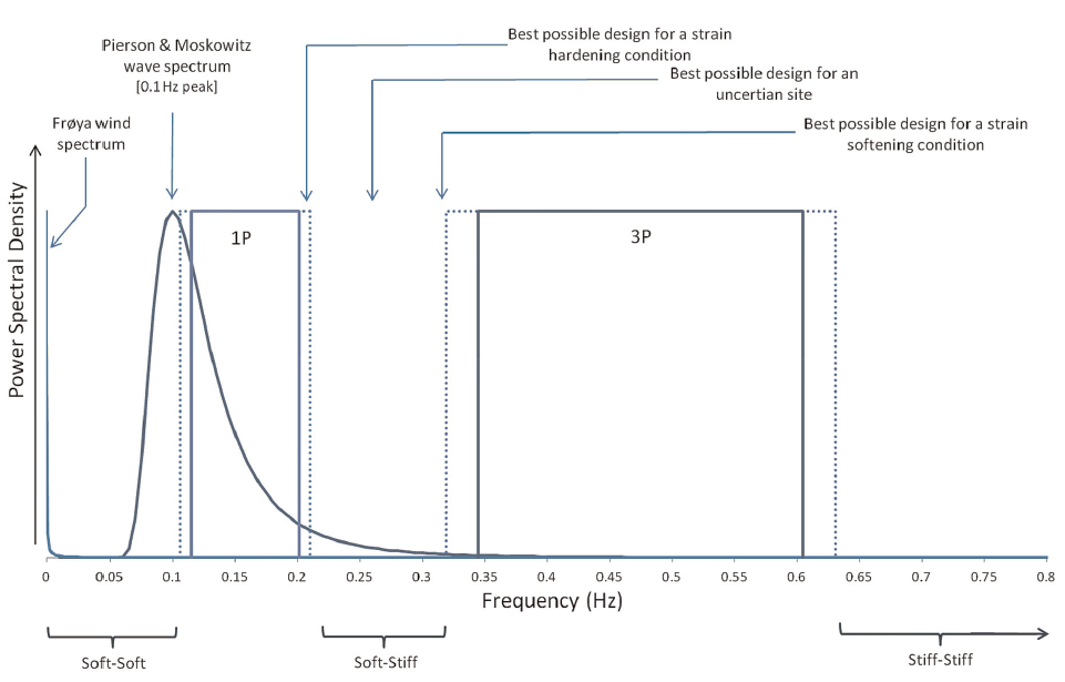
Only static structural analysis was carried out. That means that all loads are supposed to be constant. In fact, the nature of almost all loads is dynamic - the values are variable over time and cause dynamic loads on a structure. It is important to verify a design of the whole structure and compare structure's natural frequencies with these of excitation forces. If the values coincide, the possibility of fatigue damage increases due to resonance. Figure 22 shows the spectrum of frequencies for the wind, wave and wind turbine's rotor. To avoid resonance, the natural frequency of the structure has to be outside the ranges of excitation forces [1].
The most problematic are the frequencies of rotors (of both wind and tidal turbines), as they are close to structure's first natural frequency (f0). There are 3 ways (see the bottom of the picture) to design the structure:
- soft-soft - f0 below 1P (rotor frequency), flexible structure
- soft-stiff - f0 between 1P (rotor frequency) and 3P (blade shadowing frequency), currently the most common method
- stiff-stiff - f0 above 3P (blade shadowing frequency), stiff structure
The safest solution, which unables resonance, would be designing the structure to be in the stiff-stiff area. However, such a construction requires a firm foundation, which increases the mass and costs. Hence, the soft-stiff method is widely used. Although it is economically viable, it is vulnerable to alterations of f0 [1]. An approach that the natural frequency shall be within the soft-stiff range has been assumed. To confirm it, the first natural frequency of the structure was calculated using modal analysis.
Analysis
As the geometry was known, the loads were calculated and constraints found, the finite element analysis was conducted. ANSYS APDL Mechanical 17.1 was used to carry out the calculations. Two base load cases were used to enable a comparison. As the design of the construction was not being verified, an approach to obtain not higher stresses in HOWaT structure was adopted. As a result, it was decided to modify the structure to fulfil this condition. Table 6 presents the considered load cases.
| Load case | Description | Loads | ||||||
|---|---|---|---|---|---|---|---|---|
| Dead Load (OWT) | Dead load (tidal) | Drag (Wind) | Drag (Waves) | Drag (Current) | Thrust (Wind) | Thrust (Tidal) | ||
| LC0 | OWT without current | |||||||
| LC1 | OWT with current | |||||||
| LC2 | HOWaT | |||||||
Two base load cases were considered, as OWTs would preferably be installed in waters with low currents (L0)- to reduce the loads. Nevertheless, when considering particular location with high tidal currents it is necessary to take into account this load (L1). For hybrid device all loads were applied.
Model description
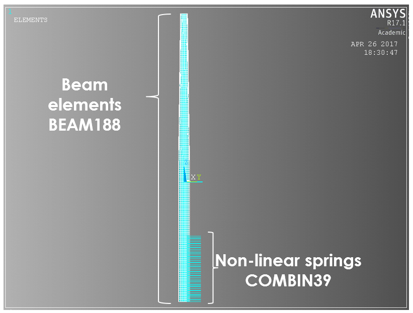
The model consits of two types of elements - non-linear springs representing soil-pile interaction and beam elements representing the monopile and the tower. Beam elements had 2 properties - for the monopile and the tower, whereas each spring had different properties, reflecting corresponding p-y curve values.
An additional constraint on the bottom of the monopile was added - the node was fixed. Figure 23 shows the model.
The loads, as calculated above, were applied to the model. Some of them, were applied as point loads (on nodes), other were applied as distributed loads (on elements).
Results
Structure
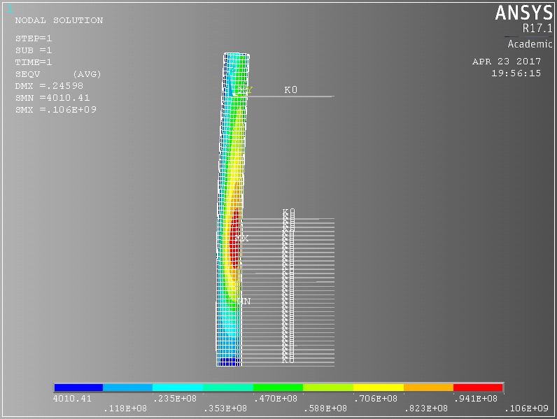
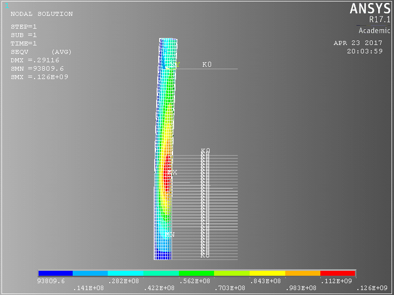
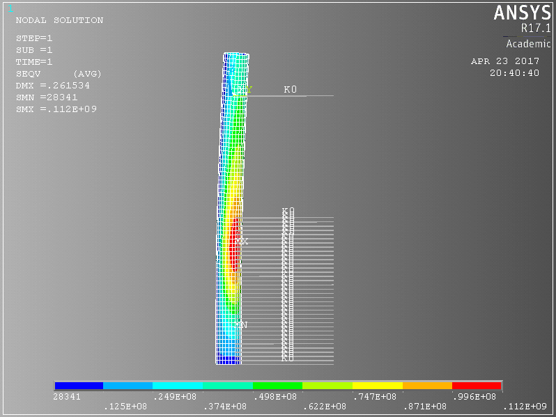
The values of Von Mises stresses were obtained. Table 7 shows the values of the stresses for each load case, whereas Figures 24.-26. plots the FEA output (note the single spring at sea level was used to illustrate that level only, its stiffness was negligible).
Von Mises stress is higher for LC1 than for LC0, whereas that of LC2 is the highest. The difference between HOWaT and OWT with current is 10.5%. Stress in HOWaT's monopile are 18.5% higher than that of OWT's foundation.
| Load case | Description | Stress | Difference |
|---|---|---|---|
| [MPa] | to HOWaT | ||
| LC0 | OWT without current | 106 | 18.9% |
| LC1 | OWT with current | 114 | 10.5% |
| LC2 | HOWaT | 126 |

As above mentioned, the goal of structural analysis was to find the impact of additional loads on structure and modify it appropriately. The simplest solution is to alter dimensions of the monopile (diameter or thickness). As soil-interaction model was developed for a pile of 6 metres diameter, modification of the dimension would result in different spring parameters. Hence, thickness modification was chosen. Additionally, it precludes local buckling in a pile [15]
Table 8 shows additional load cases - taking into account thickness modifications to fulfil two base load cases (LC2_A1 is compared to LC1, while LC2_A0 was compared to LC0). Figure 27 and Figure 28 show FEA analysis for those altered monopiles.
| Load case | Description | Stress | Comparison |
|---|---|---|---|
| [MPa] | to base LC | ||
| LC0 | OWT without current | 106 | |
| LC1 | OWT with current | 114 | |
| LC2 | HOWaT (70 mm) | 126 | 118.9% / 110.5% |
| LC2_A1 | HOWaT (80m m) | 112 | 98.5% |
| LC2_A0 | HOWaT (8 mm) | 106 | 100% |

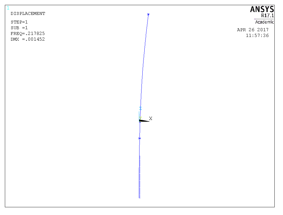
Natural Frequency
The same software was used to calculate natural frequency (f0) of the structures (as described in Table 9).
The obtained values (Figure 29 shows a sample solution for one of the structures) are similar - the influence of attaching additional structures to the monopile and increasing the pile thickness is insignificant. It is worth to mention, the value of f0 was slightly increased due to modifications.
| Load case | Description | Tidal Structure | Frequency [Hz] |
|---|---|---|---|
| LC0 / LC1 | OWT (70 mm) | 0.21670 | |
| LC2 | HOWaT (70 mm) | 0.21783 | |
| LC2_A1 | HOWaT (80 mm) | 0.22458 | |
| LC2_A0 | HOWaT (85 mm) | 0.22757 |
The obtained values were compared with the range of frequencies of wind and tidal rotors. Table 10 presents the characteristics of rotors and frequency ranges. Those values are also shown in Figure 30.
| Device | Lower rotor speed | Upper rotor speed | ||||
|---|---|---|---|---|---|---|
| Speed | Frequency 1P | Frequency 3P | Speed | Frequency 1P | Frequency 3P | |
| rpm | Hz | Hz | rpm | Hz | Hz | |
| Wind turbine | 6.9 | 0.1150 | 0.3450 | 12.1 | 0.2017 | 0.6050 |
| Tidal turbine | 4.0 | 0.0667 | 0.2000 | 11.5 | 0.1917 | 0.5750 |
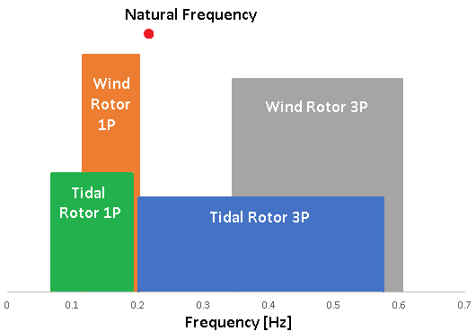
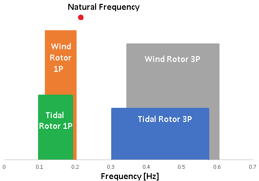
The natural frequency of HOWaT's structure overlaps the tidal turbine frequency range (that of blade shadding). This can result in high vibrations of the structure due to resonance effect. Moreover, modification of the f0 would not solve the problem within soft-stiff region, as there is no such a range when wind and tidal turbines are combined.
To resolve this vibration issue, a modification of rotor's characteristics was proposed. Increasing the lower rotor speed to 6 rpm would result in sufficient soft-stiff range for the structure. However, such an approach can reduce the efficiency of the tidal turbine and its energy output. Redesign of blades or controlling system could be mandatory to optimise power coefficient and keep low cut-in speed.
The influence of this alteration was not taken into account in our project. We assumed the turbine characteristics were not changed.
Conclusions
The structural analysis allowed us to determine the impact of tidal structure on a monopile. Additionally, potential vibrational issues were found, based on natural frequency calculations and turbines' characteristics. The solution for reducing structure's vibration was proposed. Below, there is a summary of our findings related to structural and vibration analyses.
Structure
The structural analysis confirmed the increased loads results in higher stresses within the foundation. The influence was not very significant, however, it cannot be neglected. Structure reinforcement was proposed (increasing thickness) to reduce the level of stresses below these of base load cases.
As the modification had a moderate size, the mamufacture technology of a monopile would not be drastically modified. It can be assumed that the cost-weight ratio would not be affected. That led us to the conclusion that the increased weight of a foundation for HOWaT would result in correlated fashion cost rise. The weight would be proportional to the monopile's cross section area. The values for different thicknesses of the pile are shown in Table 11.
| Thickness (mm) | Area (m2) | Relative to 70 mm |
|---|---|---|
| 70 | 1.304 | |
| 80 | 1.488 | 114% |
| 85 | 1.580 | 121% |
Frequency
The investigation of possible vibrations within the structure indicated one of the most important challenges of our concept. Because the nature of tidal and wind turbines are different, their parameters are varied as well. That can result in a wide range of combined operating rotational speeds. This results in narrowing or even removing soft-stiff area. Thus, another way of designing the foundation must be adopted (soft-soft or stiff-stiff). Alternatively, the design of turbines used must take into account the attributes of the other device to expand the soft-stiff range.
- Bhattacharya, S. (2014). Challenges in Design of Foundations for Offshore Wind Turbines. Engineering & Technology Reference.
- Jonkman, J., Butterfield, S., Musial, W., & Scott, G. (2009). Definition of a 5-MW Reference Wind Turbine for Offshore System Development.
- Jonkman, J.,Musial,W. (2010) Offshore Code Comparison Collaboration (OC3) for IEA Task 23 Offshore Wind Technology and Deployment, Technical Report NREL
- Marine Current Turbines, SeaGen-S 2MW Brochure
- Det Norske Veritas (2014) DNV-OS-J101 Design of Offshore Wind Turbines.
- British Standard Institution (2009) BS EN 61400-3:2009 Wind turbines - Part 3: Design requirements for offshore wind turbines
- Facts and figures - Belwind http://www.belwind.eu/en/facts-and-figures/
- European Committee For Standardization (2010) EN 1991-1-4:2005+A1:2010 Actions on structures - Part 1-4: General actions - Wind actions
- British Standard Institution (2011) NA to BS EN 1991-1-4:2005+Al:2010 UK National Annex to Eurocode 1 - Actions on structures Part 1-4: General actions - Wind actions
- Clarke, J. (2016) Course Material on Wind Energy. ME927 Energy Resources and Policy, University of Strathclyde
- Ingram, G. (2011) Wind Turbine Blade Analysis using the Blade Element Momentum Method. Version 1.1
- Det Norske Veritas (2010) DNV-RP-C205 Environmental Conditions And Environmental Loads
- Fugro GEOS (2001) Wind and wave frequency distributions for sites around the British Isles, for the Health and Safety Executive
- Tezdogan, T. (2017) Course Material on Wave kinematics. NM969 Marine Renewable Energy Systems, University of Strathclyde
- American Petroleum Institute (2003) Recommended Practice for Planning, Designing and Constructing Fixed Offshore Platforms—WorkingStress Design
- Passon, P. (2006) Memorandum: Derivation and Description of the Soil-Pile-Interaction Models