
Output
This page details the research, methodology, assumptions and inputs which created the tools to analyse the power output implications of adding PV panels to an existing wind farm. Results of the different analyses carried out are given, followed by discussion of the implications of the outputs and how this influences the technical feasibility of integrating PV and Wind.
Use menu above to move directly to any of the sections of interest. There is a link to a “sample power calcs” spreadsheet in the Results section which gives the opportunity to add your own Wind Farm output data, irradiance data or vary turbine or PV panel parameters to generate your own outputs and perform your own analyses. There is an additional “analysis data” spreadsheet from the project available for download in the Results section if you wish to interrogate the project outputs yourself.
Research
Determining current knowledge
Initial research from a literature search revealed that previous investigation of the concept of combining Wind and PV generation had been on a small scale in discrete, islanded models where the output was used directly at that particular location, often in conjunction with battery storage. There was no evidence of research utilising combined power generation sources in a grid connected mode.
Turning attention to practical aspects of the project, it was important at the outset to understand the characteristics typical of a commercial windfarm found in the UK in terms of location, capacity and type/size of wind turbine utilised. The website www.variablepitch.com holds the details of all renewable energy generation installations registered under government renewable subsidy schemes. The information held here on Wind generators was used to determine that a farm of 10 individual 2MW turbines would be a reasonable model to use to base calculations and analysis on.
A number of manufacturers produce 2MW wind turbines with similar output characteristics. For the purposes of modeling, a Vestas V90 model was selected, as the power curve data (lookup table) was readily available for use.
In order to provide as accurate an analysis of energy outputs as possible, it was determined that wind and solar data was required at as small a time resolution as it was possible to obtain. Extensive research revealed that detailed hourly or 30 minutely data for a wide spread of UK locations was theoretically available from various international sources, gaining access in a timely or cost free manner proved unfeasible. Therefore use of freely available hourly climate data from ESP-r was the most realistic option for the project.
Back to top
Assumptions
Justification of Calculation Inputs Used
Consideration was given to which physical locations should be used to best test the concept. Ideally this would be somewhere where there was both a reasonable level of wind and solar resource and existing wind farms which would be representative of the 10 x 2MW turbines previously identified as representative. This detailed match was not possible as climate data was restricted to that available in ESP-r. Interrogation of graphic wind and solar resource maps identified Hemsby in Norfolk as the single location which best matched these objectives. However, data was also obtained from the remaining ESP-r locations in the UK to enable checking of a range of climate types.
Real measured hourly climate data taken from ESP-r was used for evaluation and analysis. The wind speed information was “raw” data from measurement stations at a 10m height above the ground. Standard height correction equations were used in order to calculate representative wind speeds at realistic turbine hub heights. This is because wind speed felt by the wind turbine blades is significantly different to that measured at standard telemetry stations due to the drag effect of the ground which diminishes with height.
For the purposes of this investigation, losses due to changes in wind direction were not calculated. A blanket 15% loss factor (as typically used by industry at the initial stages of wind farm design) on turbine output was added late in the project, although all the sensitivity analysis work and site comparison analyses were completed without taking this loss factor into account. The hourly data given by ESP-r was assumed to remain constant across the hour and therefore able to represent both an instantaneous power value and cumulatively, energy delivered. This was true for both the wind and solar outputs generated
Following review and comparison of a number of different methods of converting location and irradiance information into irradiance levels hitting an inclined panel, step by step calculations were extracted from www.pveducation.org. The details of which can be found here. Part of the attraction of PV technology in the UK is that it can utilise both direct and diffuse solar radiation. As the UK does not benefit from high levels of direct solar radiation due to its global latitude, ensuring that calculations captured the contribution from diffuse solar radiation was critical to provide representative outputs.
Advice suggested that for fixed pitch solar panels, it was reasonable to assume an angle of 30 degrees to the horizontal for the UK. Loss factors of 10% were applied to the calculated PV outputs to wrap up system and shading losses. This was validated by the Shading analysis which confirmed that output losses due to shading (assuming panels placed in a favorable part of the field) were of a small order of magnitude and would not significantly impact on the economic value of the electricity generated.
PV panel side and effective area was investigated through manufacturers data sheets. For a typical 250W panel, manufacturers all claimed generation efficiencies of around 15% and it was this efficiency which was used for the detailed final analysis work. Sensitivity analysis considered generation efficiencies in the range of 10 to 15%.
For the purposes of assessing PV capacity factor, there are a number of measures commonly in use which reflect the fact that PV panels can only possibly be generating electricity during daylight hours.
Back to top
Success criteria
Determining desired outputs
For integrated wind and PV generation to demonstrate full technical feasibility it was determined that the following criteria should be demonstrated through the combined power output calculations:
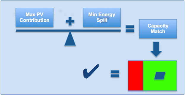
Diagram of Success Criteria: Seasaw of balanced Max PV Contribution + Min Energy Spill = Capacity Match. Add PV area is green = tick
Back to top
Boundaries
Bounding the limits of the analysis
The following boundaries were applied to the analysis in the spreadsheet. It is possible to perform additional variations if desired to investigate further aspects of the concept.
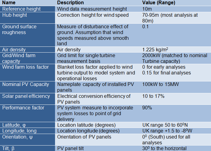
Analysis definitions and parameter boundaries - Input variable definitions and analysis boundaries
Back to top
Calculations & analysis – results
A sample analysis spreadsheet can be downloaded from here. This is preloaded with Hemsby data and will allow editing to allow the user to load in their own turbine and climate data to perform matching analysis for their own particular circumstances. Climate data from the available ESP-r UK sites is available here for use in the analysis spreadsheet
Sample results from the spreadsheet are available by clicking here. There are results from Hemsby, Oban and Porto for a range of different capacity sensitivities for interrogation if further detail is desired beyond the results below.
For example, a fundamental requirement for success of adding PV to existing Wind generation is that there is sufficient physical land area available. The calculations revealed that for 2MW of PV matched to 2MW of Wind capacity 7.79% of physical land space between the turbines (on minimum spacing) was required for the PV generation. This does not take into account array spacing, inverters etc… but illustrates that the space required is well within the area available. Further details can be found be interrogating the results in the spreadsheet linked above.
An illustration of the fundamental principles of “filling the gap” are shown in the two graphs below. The first is wind output only. It is extremely spikey and there are considerable gaps between the output and the grid connection capacity (red line). Adding in PV generation as shown in the orange graph below preserves the spikey nature of the output. However, it does even out some of the output gaps, particularly in the summer months. It also results in numerous instances with extra tall output spikes where generation exceeds the grid capacity limit. This excess generation must be spilled and is therefore wasted generation.
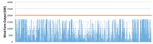
Graph of hourly Wind Farm output variation across an entire year
Illustrated below is how PV power contributes to the total site generation and the amount of this energy with has to be spilled as the installed capacity of PV increases. The aim is to maximise PV contribution whilst minimising spilled power. Unfortunately, due to wind and PV positive correlation, as PV begins to make a significant contribution to overall generation, the proportion of spilled power increases more rapidly. This results in additional PV contribution begining to level off and the proportion of power spilled increasing as more PV is added. This is particularly noticeable as PV installed passes turbine rating – doubling PV increases its contribution from 25 to 40%, but spillage dramatically increases from 1.6 to 8.2%.
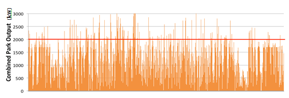
Graph of hourly combined generation output variation across an entire year
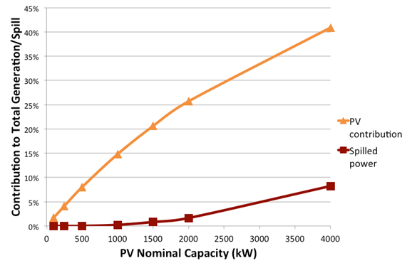
Graph of increasing PV contribution to generation and power spill with increasing nominal PV capacity
Variation in PV Contribution and Spilled Output with Nominal PV Capacity Installed. Sensitivity analysis to determine the effects of increasing ratio of PV:Wind installed capacity. For a 2MW wind turbine (15% turbine loss factor) installed in Hemsby
PV technology has improved for commercial panels in recent years, so it was important to understand how sensitive outputs were to the efficiency of the PV panels. Results of this sensitivity analysis are shown in the table below. Contribution to generation is significantly more sensitive to improved efficiency than spill is. Therefore, to improve the financial case and give the largest possible contribution, it is important to use the most efficient PV panels available.
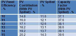
PV Efficiency Sensitivity: Hemsby, 80m Turbine hub height, 2MW Nominal PV
Wind farm design is extremely sensitive to turbine hub height. The aim of developers is usually to maximise the hub height of turbines within the constraints of planning requirements in order to benefit from higher wind speeds further from the ground. The table below shows that the matching of Wind to PV is not particularly sensitive to variations in turbine hub height. This is the case for both Hemsby and Oban.
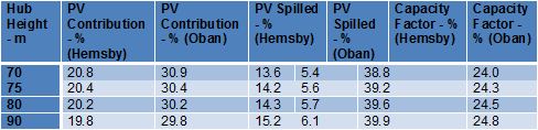
Hub Height Sensitivity: Hemsby, 15% PV Efficiency, 2MW Nominal PV
Having determined that 80m hub height and a nominal 2MW of PV capacity was a reasonable way to even out some of the spikiness in combined generation without generating too high a level of excess power to be spilled, the remainder of the results will focus on this scenario.
Comparing Hemsby and Oban in the table below, it is clear that outputs generally in Oban are lower. Surprisingly, the contribution to the combined generation from PV is actually higher in Oban. This is mainly due to the poor levels of wind present in the data which was available for this study. It is likely that the actual wind speeds will be higher in the north west of Scotland and therefore the proportion of energy supplied by PV will actually be lower in practice.
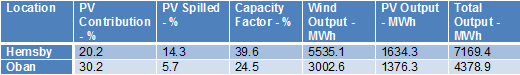
Comparison of Annual Outputs at Hemsby and Oban: 80m Turbine hub height, 2MW Nominal PV, 15% Efficiency, No Turbine Loss Factor
Looking in further detail, monthly generation during January and June for both locations is given below. Wind generation is noticeably more dependable in Hemsby, particularly during January when there is little PV available. There appears to be very little wind output in Oban during June which allows the PV generation to dominate.
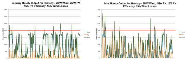
Hemsby January and June Outputs: 2MW Turbine, 2MW PV, 15% PV Efficiency, 15% Wind Losses
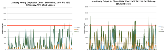
Oban January and June Outputs: 2MW Turbine, 2MW PV, 15% PV Efficiency, 15% Wind Losses
Focusing further in, the remaining results will concentrate on the Hemsby case as this is most representative of a real live site where co-generation might be considered. The table below gives data on monthly statistics for a 2MW Turbine with 2MW of nominal PV. As climate data predictions would lead us to except, PV has a far larger contribution (with associated energy spill) to total generation during the summer. The large amounts of spill experienced would cause significant control and metering problems for the developer feeding into a nominally fixed capacity grid connection and add significantly to the cost of control of the entire site.
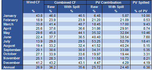
Monthly Capacity Factors, PV Contribution and Spill for Hemsby
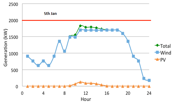
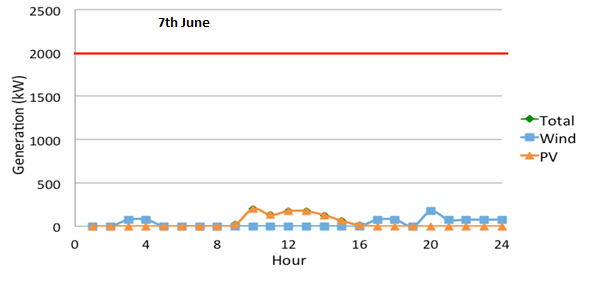
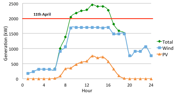
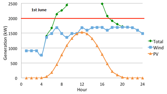
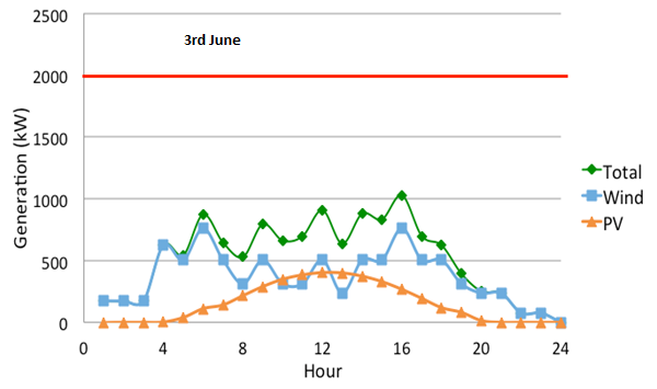
Some fairly typical hourly combined outputs for individual days are shown in graph form below to demonstrate the difficulties in filling the generation gap. The red line in each case is the connection capacity. 5th January is dominated by wind output, with virtually no PV contribution. The high wind output mainly in daytime hours with little wind during the night. 7th January is a write-off. There is virtually no output from either source. As you move into Spring months, you start to experience windy days which are also sunny. 11th April illustrates this clearly. Energy spill becomes significant and total output drops off at night. This effect is exaggerated in summer when solar levels are potentially at their highest. At midday on 1st June, more than half the output is above the grid connection capacity limit and would have to be spilled. However, even in the summer, solar resource is unreliable and you can’t guarantee you can offset it with wind production. June 3rd demonstrates this clearly with low levels of output from both wind and PV through the whole day and again, wind dropping off at night.
Interpretation of results - conclusions
To summarise – there are huge variations in daily and hourly outputs of both wind and PV which make determining a nominal PV capacity to match Wind output unrealistic. Wind output generally dominating in the winter, although it is unreliable and tends to drop off at night. PV addition can result in significant energy spill in the summer. This negates any positive impact from improved generation output contribution. PV output is also unreliable.