

B.E2 Results
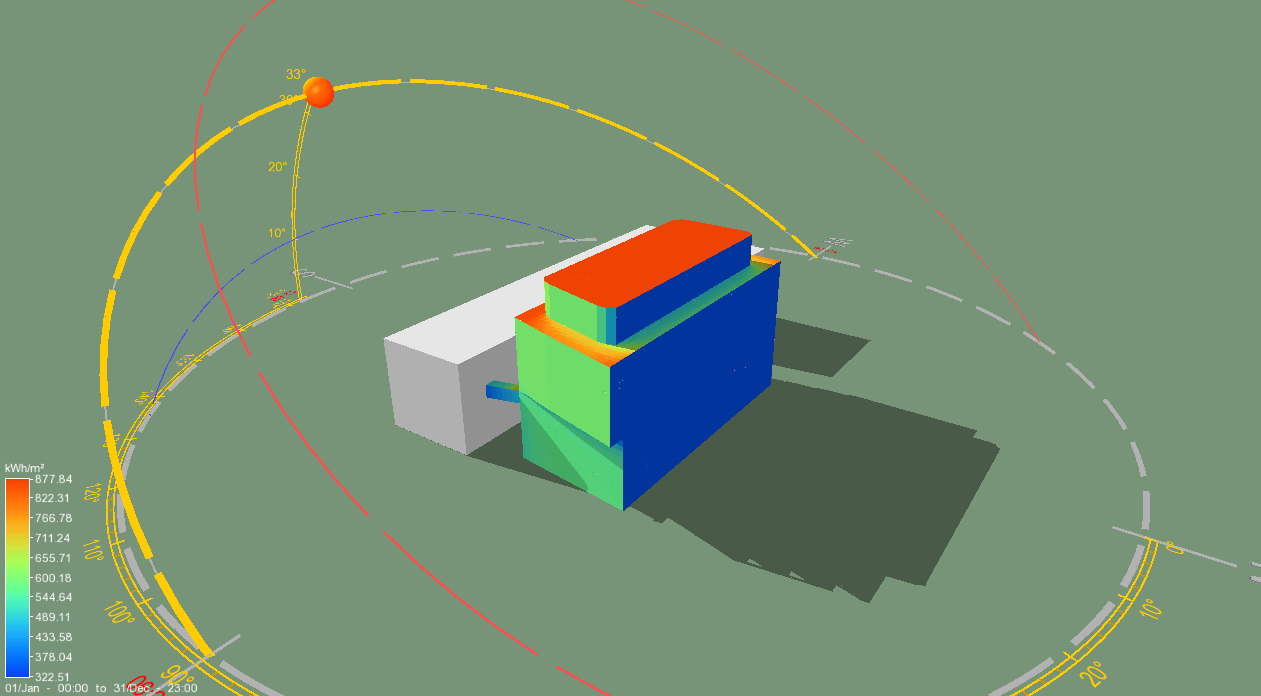
The tables and graphs below show the improved energy consumption and improved levels of comfort as the result of experimentation using dynamic building simulation. The results also show CFD run outputs for office space, highlighting cold wall effects in the base case. It can be seen, based on the two simulation results, that there is an energy saving of about 6.90%.
The comparison of the metered data to the simulated data is given in figure-3. The BMS data is made up of data recorded by the ES before this project was started(October, November and December) and data that has been extracted from the BMS in this project (January, February, March and April). Calibration (validation of) the model would have obviously been required to meaningfully compare the simulated results to the BMS (metered) data. It was however, not attempted for the project due to its [the project] short time frame.
Overall Energy Consumption
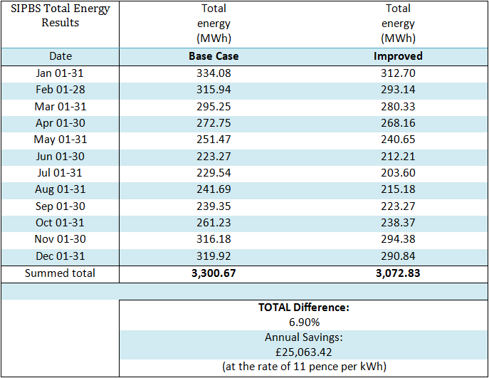
The monthly overall energy consumption of the SIPBS building is shown in table 1, it also shows the overall cost saving.
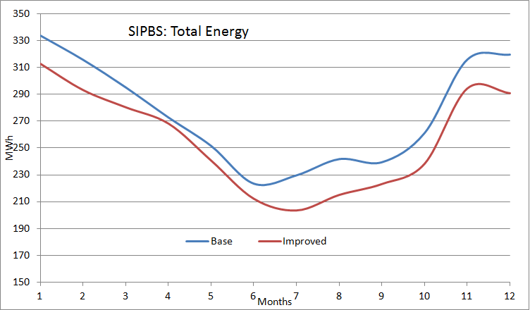
The total energy consumption of the SIPBS building is shown in figure 1.
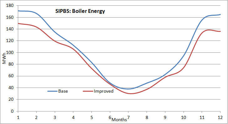
Boiler Energy Consumption
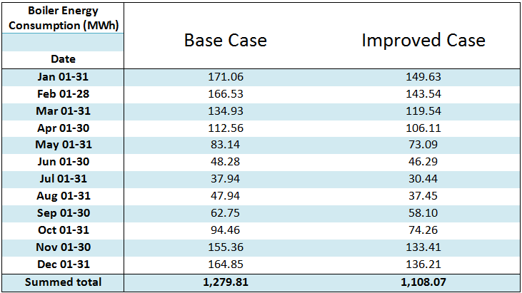
The monthly boiler energy consumption is shown in table 2.
The boiler energy consumption is graphed in figure 2.
Metered (from BMS) boiler gas consumption vs Simulated
The actual boiler energy consumption compared to the trened BMS boiler energy consumption is shown in figure-3. The BMS data came from two sources: data gathered by ES from BMS for the months of: October, November and December; and trended data extracted from BMS for the purpose of this project for the months of: January, February, March and April.
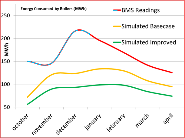
As can be seen in the figure, the data in the first section of the graph is not only considerably different (see the pick in BMS readings - figure-3 above) from the simulated data but also appears to be out of phase. This could be a result of one or a combination of the following issues: a wrong BMS sub-meter reading by ES, BMS malfunction, AHUs malfunction, Boiler malfunction or lack of calibration of the simulation model. As mentioned previously, model calibration would have helped to further match modelled building energy consumption to real energy consumption (metered) but limitations of available BMS data and the duration for the project made this improbable.
Chiller Energy Consumption
The monthly chiller energy consumption is shown in table 3.
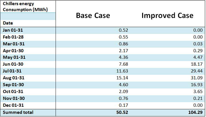
The chiller energy consumption is graphed in figure 4.
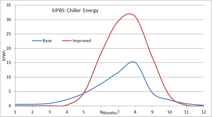
Annual chiller energy consumption shows significant increase during late spring, summer and autumn months. It is worth mentioning that in July and August the teaching labs are mostly unoccupied, and hence the real energy consumption would probably have been much lower, as the chillier operation would not be required (real occupancy rate is unknown or unpredictable).
Due to lack of clear occupancy statistics during these periods, occupancy profiles similar to the teaching periods was assumed for the spaces.
Office Zones Heating Loads Compared
Figures 5 and 6 show the office zone boiler loads for August and January


Office Zones Comfort Levels Compared
Figures 7 and 8 show the office zone comfort levels for August and January


Office Zones Mean Radiant Temperature Compared
Figures 9 and 10 show the office zone radient temperatures for August and January


Teaching Labs Heating Loads Compared
Figures 11 and 12 show the teaching labs boiler loads for August and January

The boilers energy consumption for the “improved” case is lower than for the base case due to optimised ventilation rate for reduced load during the night hours.

Teaching Labs Comfort Levels Compared
Figures 13 and 14 show the teaching labs comfort levels for August and January


Teaching Labs Zone Temperature Compared
Figures 15 and 16 show the teaching labs zone temperatures for August and January


CFD Result
Figure 17 shows the CFD of the office zones and its resultant temperatures.
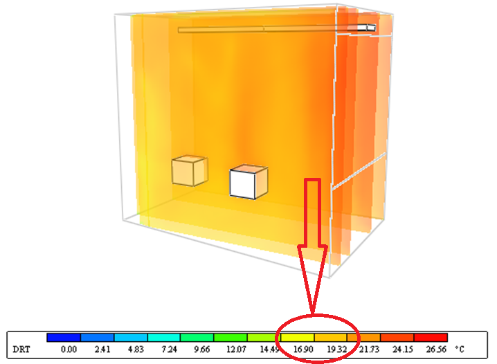
The zone, presented as yellow and light orange colour, indicate where dry resultant temperatures are between 16.9 and 19.32oC, which could be experienced as too low a temperature for office type activity.