SIHEEBEP
Study of the Impact of Home Entertainment Equipment on Building Energy Performance

 

RESULTS

Winter simulation (comfort metrics, heating requirements , CO2, Cost) |
Summer simulation (comfort metrics, cooling requirements, CO2, Cost)

The results obtained from the simulations carried out for the three situations under analysis are shown below in terms of:

• Temperature and thermal comfort metrics
• Heating and cooling requirements
• CO2 emissions
• Cost

Results are shown independently for both the winter and the summer simulation.
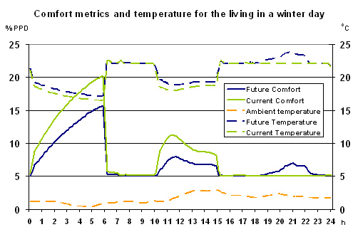
Specific graphs for the living are shown, as it is considered to be the most representative zone within the house.

Winter Simulation

• Temperature and comfort metrics

The comfort metrics from the current and the future situation are shown for the living in a winter day in figure 1 below. Thermal comfort is evaluated in terms of the percentage of people dissatisfied (%PPD).

Figure 1. Comfort and temperature metrics for the living in the current and future situation

Analysis:

We can clearly observe the effect of the heat gains from the devices  in the comfort metrics of the house. When the heating system is not working (10am-15pm and 0pm-6am) the future temperature inside the house is about 2ºC higher due to the greater heat gains from the future home equipment, with 5% less of people dissatisfied right before the family wakes up at 6am. In addition to this, it is remarkable how the heat gains from the future situation rise temperature from 19pm to 22pm, while many devices are working and hence reducing comfort. However, the heating system is working at that time in the current situation as the lower casual gains are not enough for meeting the heating set point of 22ºC. This issue will be further analyzed in the next section.

Back to top

• Heating  requirements

Heating system details:
Working hours: 6am-10am / 15pm-24pm
Heating set-point: 22ºC

Graphs
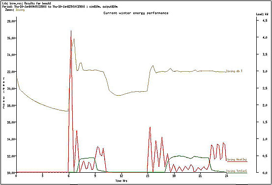
The energy performance of the living for a winter day is shown in the following graphs:

Temperature: brown line
Casual gains: green line
Heating loads: red line

• Current Situation


Figure 2. Living temperature, casual gains and heating requirements

 

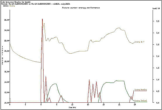
• Future Situation

  
  Figure 3. Living temperature, casual gains and heating requirements

 

• Rational Situation

  
  Figure 4. Living temperature, casual gains and heating requirements

Analysis:

There is a clear effect of the casual gains on both the heating requirements and the temperature metrics as we can see in the previous graphs.

We can note in figure 2(current situation) that the casual gains (green line)  appearing curb the heat requirements (red line) significantly, however, the heating system needs to be on during all the working hours and hence the temperature is kept on the set point quite accurately.

On the other hand, the casual gains appearing on figures 3 and 4 (future and rational situation) are that high that totally eliminate the heating loads. These casual gains are big enough not only to eliminate the heating requirements but also to make temperature rise significantly over the set point, especially in the evening when it goes up to 24ºC.This phenomenon has a clear impact on the comfort metrics as we saw in figure 1. It is also remarkable how the heating loads at 6am (when the heating system starts working) are 54% greater in the rational situation than in the future one. This is due to the fact that as in the rational situation the devices are totally switched off during the night, the house cools down to 16ºC while in the future situation it cools down to 18ºC only.
Similar results are obtained for the rest of the zones inside the house.

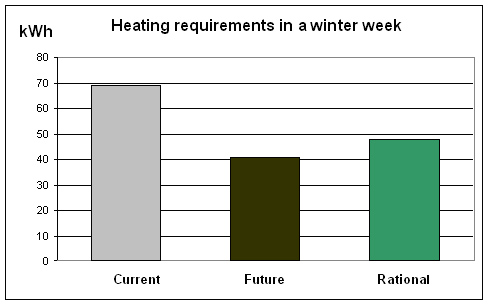
Overall analysis:

The total heating requirements of the dwelling for a whole winter week are shown in figure 5 below for the three situations considered:

Figure 5. Heating requirements for the three situations

As we can see, the heating loads decrease by 40.5 % from the current to the future situation, this is due to the greater casual gains appearing in the future situation due to the increase in home entertainment devices, which contribute to warm up the house curbing the heating requirements.

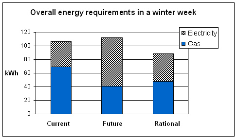
Because of the same reason, the heating loads are also significantly lower in the rational situation, however, they increase by 15% in comparison with the future ones due to the elimination of the heat gains from the standby and the off consumption.

If we consider now the overall energy analysis (shown in figure 6 below), including also the electricity requirements from the devices considered in each situation, we note that although the gas consumption decreases by 40.5%  from current to future due to the lower heating requirements, the massive increase in the electricity consumption leads to an overall energy increase of 5%.

On the other hand, and even though the gas consumption is greater in the rational situation than in the future one due to the greater heating loads, the savings in the electricity demand, which decreases by 43% due to the elimination of both the standby and the off consumption of the devices, allows the rational situation to achieve a potential energy saving of 21%.

Figure 6.Overall energy requirements for the three situations

Back to top

• CO2 emissions

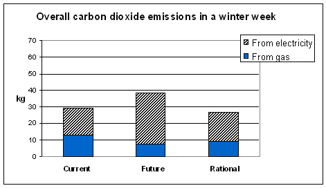
The CO2 emissions from the dwelling for the three situations are shown below in figure 7.
Emission factors considered:
0.19 kgCO2 /kWh gas
0.523 kgCO2 /kWh electricity
The emission factor considered for electricity is a rolling average factor [1], suitable for calculating emissions reductions from activities that bring about short term electricity savings (such as switching off equipment at night)

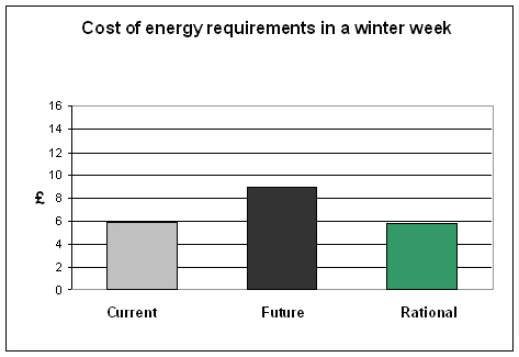
Figure 7.Overall CO2 emissions for the three situations

Back to top

• Cost

The overall cost of energy for the three situations is shown below in figure 8.
Prices considered:
2.6 pence/kWh gas
11.03 pence/kWh electricity

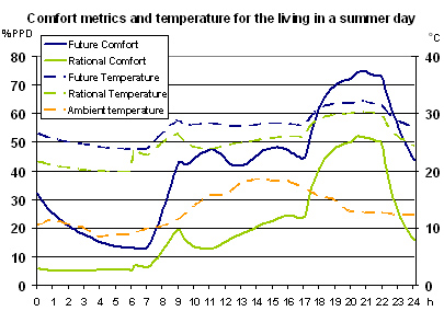
Figure 8.Overall cost of energy for the three situations

Back to top

Summer simulation

• Temperature and comfort metrics

The comfort metrics for the future and the rational situation are shown for the living in a summer day in figure 8 below. No cooling system was considered.

Thermal comfort is evaluated in terms of the percentage of people dissatisfied (%PPD).

Figure 8.Comfort and temperature metrics for the living  in the rational and future situation

Analysis:

The heat gains from the home entertainment equipment have a significant impact on the thermal comfort inside the dwelling as it is shown in the figure 8 above.

The clearest effect can be seen from 22pm to 6am: the devices are totally switched off once the family goes to bed at 22pm, and this allows the house to cool down to 20ºC in the rational situation, however, in the future one the house cools down only to 23ºC due to the casual gains from the devices kept on standby mode. This issue has a major impact on the comfort metrics as we can see in the comfort trend from 22pm to 6am.

The advantages of a rational usage of the devices can be observed again at 9 am, when the house cools down again due to the people switching off the equipment when they leave for work.

Due to this cooling processes, when people arrives from work at 17pm and many devices start to be used, the rational temperature rises up to 30ºC, while the future temperature raises up to 32ºC, both being driven by the same number of devices being used with  the same usage pattern. Again the effect on the comfort metrics can be clearly seen with a 20% more people dissatisfied in the future situation than in the rational one while they just stay at home watching TV.

Although the temperatures reached are quite high for the location being considered, we would still have to consider the possibility of using mechanical ventilation, which would actually cool down the house. Anyway a rational usage of the devices would definitely help on this issue.

Further more, and in case the installation of a cooling system was considered, a rational usage of the devices would be vital in order to curb the cooling requirements, as it will be demonstrated in the next section, where the results for a simulation with cooling system are shown:

Back to top

• Cooling requirements

Cooling system details
Working hours: 6am-10am / 15pm-24pm
Cooling set-point: 25ºC

Graphs
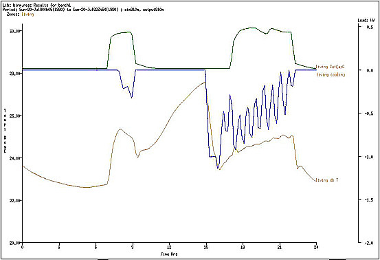
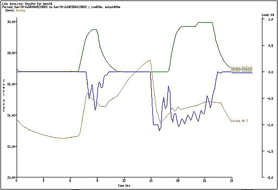
The energy performance of the living for a summer day is shown in the following graphs:

Temperature: brown line
Casual gains: green line
Cooling loads: blue line

• Current Situation

Figure 9.Living temperature, casual gains and cooling requirements

 

• Future Situation

Figure 10.Living temperature, casual gains and cooling requirements

 

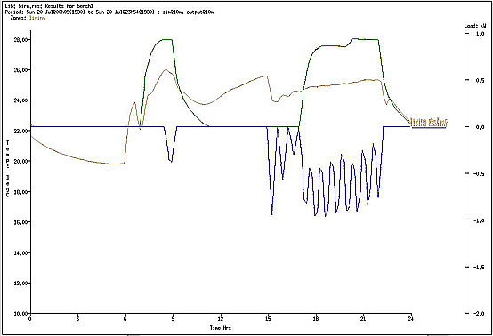
• Rational Situation

Figure 11. Living temperature, casual gains and cooling requirements

Analysis:

We can clearly observe in the previous graphs how the casual gains affect the cooling requirements. The future situation is obviously the one with higher cooling loads, due to the higher amount of devices being considered. In both the current and the future situation the house cools down only to 23ºC, and hence the temperature increases faster during the rest of the day, this is the reason why both situations require high cooling loads in the evening. On the other side, the rational situation, having the same casual gain regime than the future one, requires a lower cooling load in the evening, as the house cooled down during the night and reached the evening at a lower temperature.

Overall analysis:

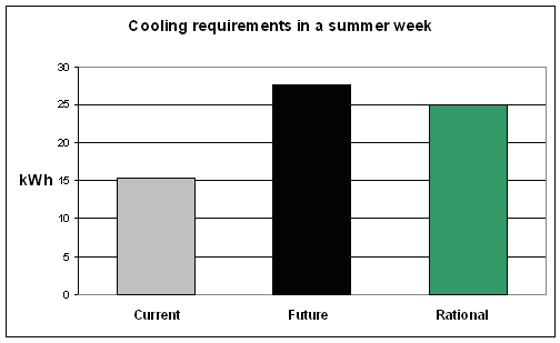
The total cooling requirements of the dwelling for a whole summer week are shown in figure 12 below for the three situations considered:

Figure 12. Cooling requirements for the three situations

As we can observe in the graph, there is a massive increase in the cooling requirements (by 45%) from the current to the future situation due to the higher casual gains from home entertainment equipment. It is remarkable how the cooling loads decrease by 10% from the future to the rational situation, showing how a rational usage can contribute to significant energy savings as it was previously mentioned.

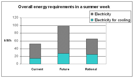
Considering now the overall energy analysis, shown in figure 13 below, including the electricity consumption from the devices, the overall energy increases by 46% from the current to the future situation.
Here is even more significant the impact of a rational usage on the energy requirements, as a potential overall energy saving of 26% can be achieved from the future to the rational situation simply by switching off all the devices when they are not being used.

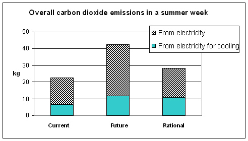
Figure 13.Overall energy requirements for the three situations

Back to top

• CO2 emissions

The CO2 emissions from the dwelling for the three situations are shown below in figure 14:
Emission factors considered:
0.19 kgCO2 /kWh gas
0.523 kgCO2 /kWh electricity
The emission factor considered for electricity is a rolling average factor [1], suitable for calculating emissions reductions from activities that bring about short term electricity savings (such as switching off equipment at night)

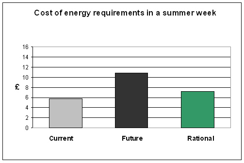
Figure 14. Overall CO2 emissions for the three situations

Back to top

• Cost

The overall cost of energy for the three situations is shown below in figure 15:

Prices considered:
2.6 pence/kWh gas
11.03 pence/kWh electricity

Figure 15.Overall cost of energy for the three situations

 

[1] Guidelines to Defra’s GHG conversion factor for company reporting, June 2007.

Back to top