• Energy Demand

• Renewables Potential

             - General Considerations

             - Specific Considerations

• Solar
  
  
• Wind
  
  
• Hydro
  
  
• Biomass
  
  
• Heat Pump

• Mabie Farm Conclusion

• Home
• Project Overview
• Opportunities
• Methodology
• Case Study
• Conclusions
• Team Members

Mabie Farm Park - Hydro

The values for the flow rate of the Mabie Farm Park stream were calculated by the Low Flows 2000 Software tool.

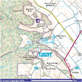
From the OS map, shown in Figure 1, the difference in altitude of the stream as it passes Mabie Farm Park is 5 m.

Figure 1. OS map, Mabie Farm Park, Dumfries

Source: Ordinance Survey

Considering that the annual Q95 flow (Environmental flow) has to be left in the stream, and by assuming a design flow for the turbine of the annual Q90 value (0.01 m³/s), the power to be produced is shown in the following table.

Table 1. Power available to be produced in Mabie Farm

	Q90 flow  (m3/s)	Environmental flow (m3/s)	Available flow (m3/s)	Flow for power generation (m3/s)	Possible Power Output (W)	Power production per month (kWh)
Jan	0.031	0.007	0.024	0.01	245	182
Feb	0.024	0.007	0.017	0.01	245	165
Mar	0.025	0.007	0.018	0.01	245	182
Apr	0.023	0.007	0.016	0.01	245	177
May	0.013	0.007	0.006	0.006	147	109
Jun	0.008	0.007	0.001	0.001	25	18
Jul	0.005	0.007	0	0	0	0
Aug	0.005	0.007	0	0	0	0
Sep	0.008	0.007	0.001	0.001	25	18
Oct	0.012	0.007	0.005	0.005	123	91
Nov	0.021	0.007	0.014	0.01	245	177
Dec	0.026	0.007	0.019	0.01	245	182

 

By comparing the supply and demand, it can be seen that the supply will represent 0.67% of the demand. The difference can be seen in the following graph:

Graph 1. Comparing Demand and Supply from Hydro in Mabie Farm

 

By considering monthly average flows and the annual average flow (0.086 m³/s) as the design flow, the results will be the following:

 

Table 2. Power available to be produced in Mabie Farm at Design Flow

	Average flow  (m3/s)	Environmental flow (m3/s)	Available flow (m3/s)	Flow for power generation (m3/s)	Possible Power Output (W)	Power production per month (kWh)
Jan	0.140	0.007	0.133	0.086	2109	1569
Feb	0.120	0.007	0.113	0.086	2109	1417
Mar	0.110	0.007	0.103	0.086	2109	1569
Apr	0.086	0.007	0.079	0.079	1937	1395
May	0.062	0.007	0.055	0.055	1349	1004
Jun	0.040	0.007	0.033	0.033	809	583
Jul	0.029	0.007	0.022	0.022	540	401
Aug	0.036	0.007	0.029	0.029	711	529
Sep	0.060	0.007	0.053	0.053	1300	936
Oct	0.100	0.007	0.093	0.086	2109	1569
Nov	0.120	0.007	0.113	0.086	2109	1519
Dec	0.130	0.007	0.123	0.086	2109	1569

 

In this case, the power production will represent an improvement, by increasing the supply and demand match as shown on the following graph.

Graph 2. Comparing Demand and Supply from Hydro at Design Flow

• This energy demand/supply profile - although more convenient - illustrates the high variability that may be found in energy production.
  
  
• Because these variations are large, it is recommended to be conservative in the prediction, recommending to consider the first case (design flow of 0.01 m³/s).
  
  
• Projecting the use of a turbine with this design flow will represent a rated power of 245 W – the equivalent of 3.5 fluorescent tubes – making it not feasible.

For achieving a better energy yield, a higher head or flow will be needed. For this, a reservoir or dam will be convenient in areas over the estate, in this case Mabie forest which is part of the forestry commission of Scotland.

In the case of installing a hydro system in this location (same head), the required flows will be:

Table 3. Flow Required to Meet Total Demand

	Required flow(m3/s)
January	0.233
February	0.253
March	0.295
April	0.319
May	0.352
June	0.415
July	0.408
August	0.395
September	0.366
October	0.328
November	0.245
December	0.243

This illustrates that the highest flow required will be during the summer when naturally the flow rates are lower.