


The loads that an offshore structure is subjected to are divided in two categories: those due to the function on the structure (Functional loads) and those due to the environment (Environmental loads). The first category includes static or dynamic loads from the operation of the structure, the weight of the structure, the buoyancy etc. The second category includes loads that come from the direct or indirect interaction of the environment with the structure, such as wind load, wave load, earthquake load, current load etc. (Mavrakos, 1999).
The two main loads that are being calculated in this project are wind load on the tower and on the rotor of the turbine and wave load on the jacket legs.
In accordance with DNV, the force due to wind that an element is subjected to is calculated from the equation:
A: projected area of the element vertical to the direction of force.
q: air pressure.
a: angle between wind direction and axis of the exposed element.
ρ: air density 1.225 kg/m3
C: shape coefficient calculated from the equation.
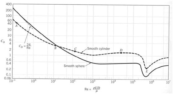
Graph 1: Shape coefficient C∞ as a function of Reynolds number
(University of Waterloo, 2005).
K: Reduction coefficient of C∞ due to finite length of the element as a function of the l/d ratio where l is the length of the of the element and d is the dimension of the cross section (height or width) measured vertically to the wind direction.
| l/d | 2 | 5 | 10 | 20 | 40 | 50 | 100 | inf |
|
|
|
|
|
|
|
|
|
|
|
|
|
|
|
|
|
|
|
|
|
|
|
|
|
|
|
|
|
|
Vtz: Average value of the wind β speed at height z m from the average sea surface for time t which is calculated from the equation:
V1hr10 Average wind velocity value at 10m height from the sea surface for 1hr time.
α, β Values used when the average time used for velocity measuring is not the same as the one for V1hr10.
| Coefficient | Average measuring time | |||||
| 1hr | 10min | 1min | 15sec | 5sec | 3sec | |
|
|
|
|
|
|
|
|
|
|
|
|
|
|
|
For the purposes of this project we have taken into consideration:
Vtz: Average value of the wind β speed at height z m from the average sea surface for time t which is calculated from the equation:
D: = 5m
L: = 90m
a: = 90deg
V1hr10 = 9m/s (so that the velocity at the top of the tower is V = 12.5m/s which is the rated power of the turbine)
and the coefficients we choose from the graphs and matrices are
α: = 1
All the other values are calculated with the equations provided.
With the aid of MATLAB program we have produced the graph of the distributed wind load along the height of the tower using the force per meter equation:
The distribution curve is as illustrated below:
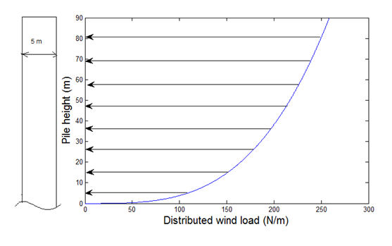
As we can imagine the force is bigger as we get higher from the sea level. By integrating the force along the height of the pile we get the total force which is Fp=3201 N.
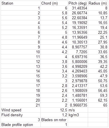
Blade profile option, 3 blade on rotor.
The output data at a rated speed of 12.5 m/s are shown below using the BEM prediction code:
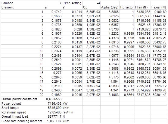
Output data using BEM prediction code.
We can see that the total force on the rotor is quite significant with its value being Fr=867771,7 N.
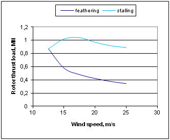
By repeating the same procedure for higher speeds we have the summarized results:
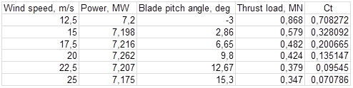
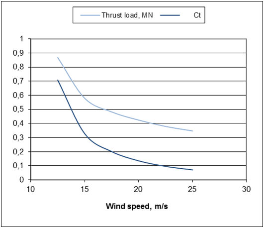
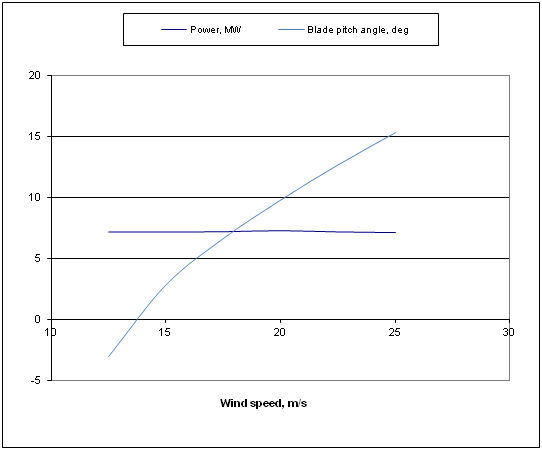
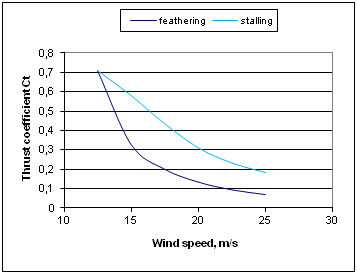
The procedure here was to operate turbine at constant rotational speed, so that tip speed ratio was adjusted as wind speed was varied. This procedure is called feathering and it is used so that maximum power is obtained at each speed. Beyond rated speed of 12.5 m/s, the blade pitch was varied to maintain power constant at about 7.2 MW (with 83% conversion of mechanical power to electrical). As we can see from the results, rotor thrust in fact reduces as a result of the blades being set to run at very small angles of attack (low lift and low drag). Thrust coefficient Ct falls dramatically as a result
(Ragheb, 2009).
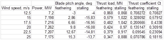
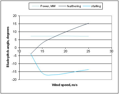
Another way of controlling wind turbines and keeping power output at the rated value when the wind speed goes up is passive stalling, where the blades turn gradually the other way and avoid the abrupt stalling as the wind speed reaches its critical value. We can see that now the thrust loading goes up as the wind speed rises, but not significantly. It increases a little and then stabilizes at a relatively high value. Thrust coefficient falls but not so dramatically as in the case of feathering. The results from the code as well as the pitch angle and thrust graphs can be seen below where we note that the thrust load for the rated speed is the same for the two approaches
(Ragheb, 2009).
cM: inertia coefficient
ρ: water density 1025 kg/m3
g: standard gravity 9.81m/s2
D: cylinder diameter
H: wave height
k: wave number which is calculated by the equation:
| shallow | intermediate | deep |
|
|
|
|
|
|
|
T: wave period where
cD: resistance coefficient
For the purposes of this project we have taken into consideration South West of England Regional Development Agency, 2006 and Coastal engineering technical note, 1985:
H = 5m
D = 1,05m
D = 40m
λ = 45,52m
Cm = 3
Cd = 1,5
All the other values are calculated with the equations provided.
Using the MATLAB program the force plotted along with the time has the following form:
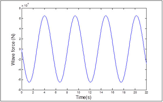
Wave force (N).
We can see that the maximum value of the wave load is Fw=65299.3 N.
By multiplying this force by 2 we will have, in approximation, the total force of the two legs at the wave front. So Fw=130598.7 N. Of course we must not forget in reality The angle of the wave may be different between these two legs, brackets will also accept significant wave forces as well as the other two legs will accept radiation forces.
Again with the aid of MATLAB program we have produced the graph of the distributed wave load along the height of the tower using the force per meter equation:
As the equation depends on time we have plotted the amplitude of the force using the transformation
The distribution curve is as illustrated below:
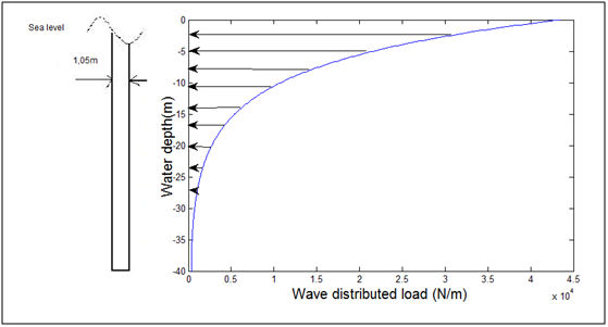
Wave distributed Load.
We can see that the maximum force is closer to the sea surface, as the amplitude of the motion decreases with depth.
The calculation of the current force will be made using the drag equation which is presented below:
where
Cd: drag coefficient as a function of Reynolds number, here taken approximately 0.38 (Graph 1)
v: kinematic viscosity of water, here taken 1,307??10?^(-6) m^2/s (The Engineering Toolbox website) at temperature of 10? (National Oceanographic Data Center website)
ρ: water density 1025 kg/m3
U: stream velocity, here taken as 1m/s uniformly distributed
A: is the reference area
So the total force along the jacket leg is Fc=8179.5 N.
As a conclusion we can say that the wave load and wind load of the rotor are of the same magnitude, but in our case the latter is about seven times bigger. The force on the pile can be considered relatively small in comparison with the others. Also, load from currents as well as wind load on the pile is comparatively not important and given the fact that it does not generate big bending moments it is not a major factor in design. So to sum up, wind load is probably the one that need to be taken into serious consideration when designing and building an offshore wind turbine.