


Analysis of the monitoring data
3 different installations have been monitored during the project. The first 2 installations (Athelstaneford and Oban) with the complete Sanyo Eco Cute system will be analysed together and studied. The particular case of the last installation (in Ballencrief) with a particular tank and 2 heat pumps will be analysed independently.
It is important to notice that the measurements of the temperature on the installations are made on the pipes. If there is no fluid circulation in the pipes, the data do not have any meaning. There could also be a small error due to the thermal conductivity of the pipes.
Data for the first two installations
The data are presented for a day where the outside temperatures for both installations are similar (between 0 and 10C). It is the 08/03/2011 for the first installation in Athelstaneford (next to Haddington) and 18/03/2011 for the installation in Oban. The daily pattern of the different curves is then quite similar during the week.
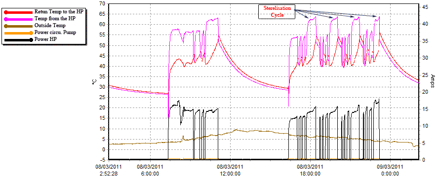
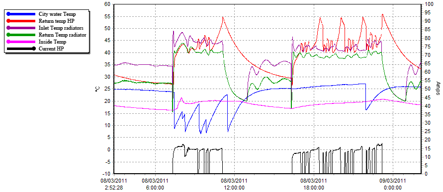
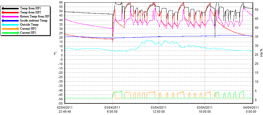
Data heat pump in the 1st case study in Athelstaneford 08/03/2011
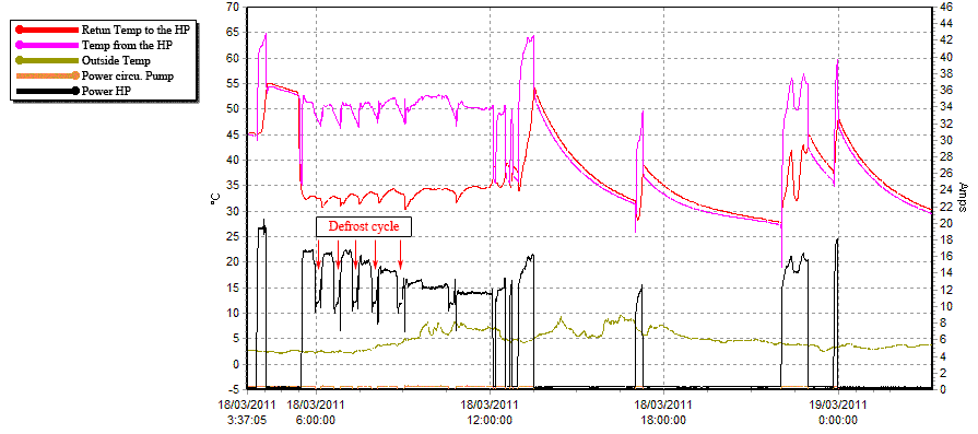
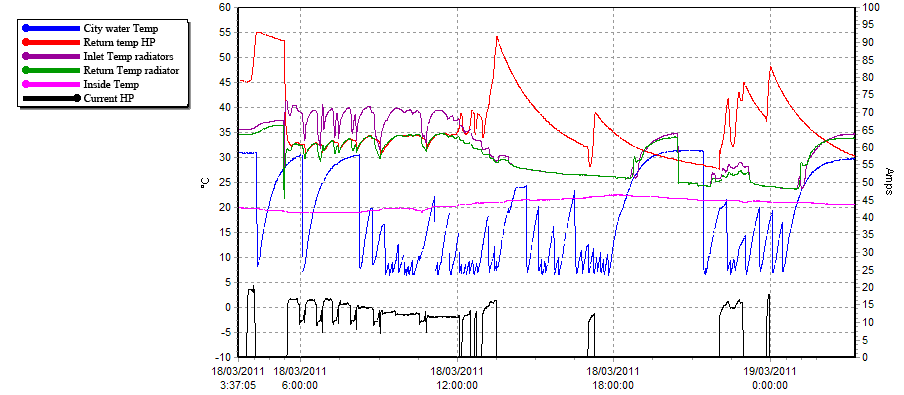
Data heat pump in the 2st case study in Oban 18/03/2011
These first graphs show the evolution of the temperature in the inlet and outlet of the gas cooler with the outside temperature and the current to the water circulation pump and the compressor. When the system is running, some hot water is provided by the outside heat pump to the tank unit.
The two systems operate in function of the periods defined in the control settings: 7-11am and 4-10pm for Athelstaneford and between 6am to 11pm for Oban. In Athelstaneford, the system is operating most of the time over the period. In Oban, the heat pump operates mainly in the morning to heat the House after the night.
The average water return temperature to the Heat Pump is lower by more than 7oC in Oban (35.1oC) than in Athelstaneford (42.5oC).
In Athelstaneford, a lot of successive starts and stops of the compressor occur, sometimes for a very short period. In Oban the number of starts and stops is a bit lower. During the afternoon there are still some operations of the device for a very short time, sometimes less than 10min.
Every 4 cycles, the system runs a sterilisation cycle: the water coming from the heat pump is heated at a higher temperature. As there are a lot of start and stop of the system in Athelstaneford, there are 5 sterilisation cycles and 3 for the day considered in Oban. In Oban, the sterilisation cycle seems to be shorter.
Data defrost cycle in the 1st case study in Athelstaneford 08/03/2011
Data defrost cycle in the 2nd case study in Oban 18/03/2011
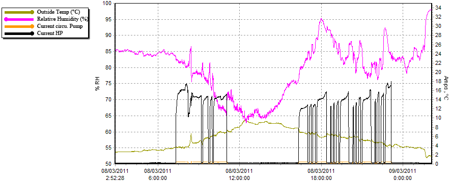
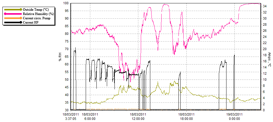
The relative humidity and the outside temperature are represented on the 2 previous graphs for both installations. The relative humidity during these 2 days in Oban and Athelstaneford fluctuates between 50 and 100%. There are 6 defrost cycles in Oban in the morning since there is a combination of low temperature and high relative humidity and the system start operating from 6am. In comparison there is only one defrost cycle in Athelstaneford because the conditions are better during the system operation.
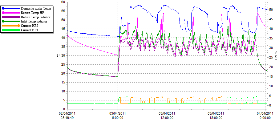
Data energy demand in the 1st case study in Athelstaneford 08/03/2011
Data energy demand in the 2nd case study in Oban 18/03/2011
The blue curves show the temperature of the water coming from the city and entering the tank. When some water is drawn, the temperature measured decreases to the actual temperature of the water coming from the city. Otherwise the measurement of the temperature increases because of the proximity of the tank. As expected, the domestic hot water demand is much higher in Oban than in Athelstaneford.
In purple and green, the temperatures at the inlet and outlet of the heating system are represented. In Athelstaneford during the night and the afternoon, the pump of the radiator is working at very low speed (high temperature drop). Otherwise the return temperature from the radiators is quite high (39.6oC on average) and the temperature drop in the radiators is quite low (around 4oC). The heating system is operating in accordance with the periods specified in the control settings. The set point of 22oC for the ambient temperature in the house is never reached over the day. In Oban the system works almost uniquely in the morning. There are some starts and stops of the radiator pump in the afternoon but at a low temperature of operation. The return temperature from the under floor heating is lower (average: 32oC) than in Athelstaneford. The ambient temperature in the house increases more slowly with the under floor heating but it is almost not necessary to heat in the afternoon.
During the system operation it can be seen in Oban that the return temperature to the heat pump is mainly determined by the return temperature from the heating system except during the sterilisation cycles. In Athelstaneford the return temperature to the heat pump is often higher than the return temperature from radiators.
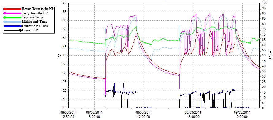
Data tank temperatures in the 1st case study in Athelstaneford 08/03/2011
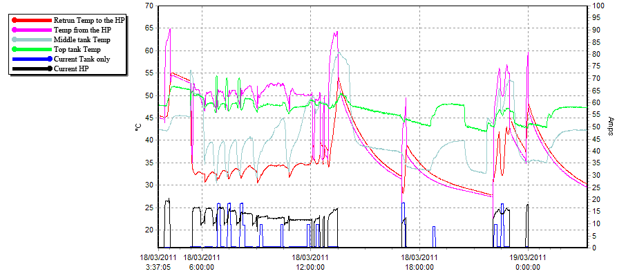
Data tank performances in the 2nd case study in Oban 18/03/2011
On the 2 graphs above, the temperatures at different heights in the tank are monitored. Considering the temperatures at the top and the middle of the tank, it can be noticed that when the heat pump is running in the Athelstaneford case, the stratification is lost. In Oban it is also the case in the afternoon when the heating system is not running, but not in the morning when the heating load is important.
Considering the current consumption of the tank, it can be underlined that the upper electric resistance is used twice in Athelstaneford and many times in Oban (2 or 4 kW).
Statistics over these 2 days
For the installations of Athelstaneford, some statistics of the main parameters are summarized on the graphs below for the 2 days of monitoring considered. The details of the calculations (excel spreadsheet) can be downloaded in the download section.
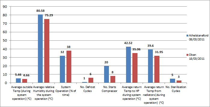
Analysis of certain parameters in Oban and Athelstaneford for the day considered
This first chart confirms the trends noticed and enables a direct comparison of both systems. There are less starts of the compressor in Oban, more defrost cycles and lower temperatures than in Athelstaneford.
The following chart contains the information on the energy consumption of the system. The voltage of the electricity supply is assumed to be constant at 230V. As it was not possible to measure the water mass flow on the installations, it was not possible to calculate directly the COP. However some estimation has been made with the regression of the COP realized with the experimental data that we had. It must however be underlined that these estimations might be slightly high since no decrease in performance is considered when the system starts and stops or is close to a defrost cycle (and the ice on the pipes degrades the performances).
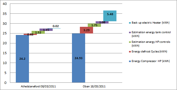
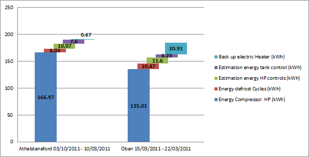
Energy consumption over the day considered
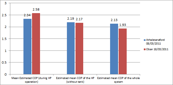
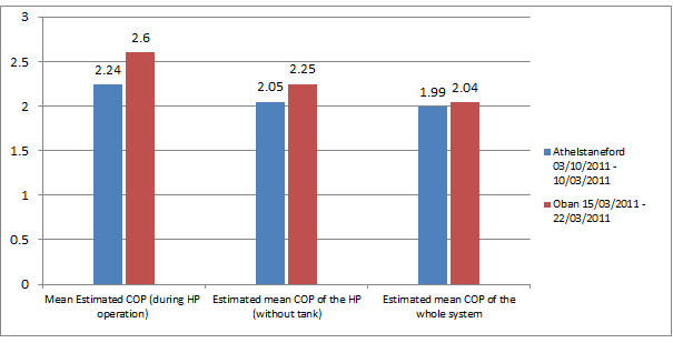
Average COP over the day considered
It can be noticed that the energy consumption of the compressor has been quite similar for both installations, but more energy is required for the defrost cycles and the back-up electric heater in Oban. It can also be underlined that the power used for the controls of the heat pumps is quite important (more than 10% of the energy used in the compressor). Considering the whole system, the energy consumption is much higher in Oban since the back-up electric heater is more used.
The average COP during the system operation is higher in Oban. However, if the energy for the defrost cycles, the controls and the back-up electric heater are considered, the COP for the installation in Oban becomes lower than that in Athelstaneford.
Statistics over the whole week of monitoring
The statistics over the same parameters have also been made for the each week of monitoring. The details of the calculations (in the same excel spreadsheet than the previous calculation) can also be downloaded in the download section.
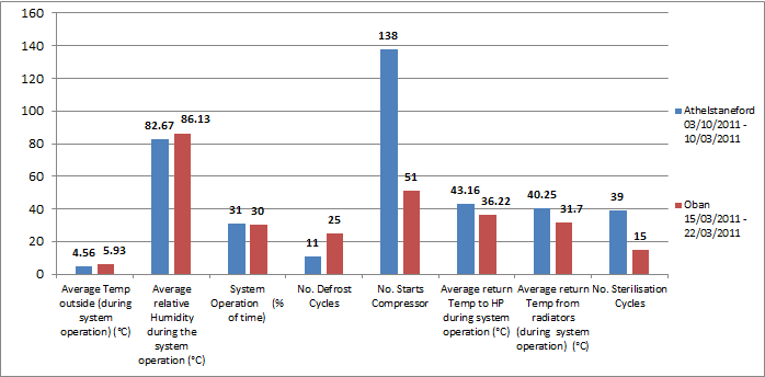
Analysis of certain parameters in Oban and Athelstaneford over the week of monitoring
The same trends for the different parameters of the parameters are confirmed. It can however be underlined that the outside temperatures was on average 1.5oC higher in Oban than in Athelstaneford over the week. In addition, the number of defrost cycles over the week for Athelstaneford is a bit more than twice what we are seeing in Oban. The ratio is a bit less important that for the unique day considered previously.
Energy consumption over the week of monitoring
Average COP over the week of monitoring
The electrical energy consumption for the heat pump is 12% lower in Oban than in Athelstaneford while the estimated heat produced is in reality only 4% lower in Oban. The mean COP of the heat pump alone (considering all the energy required for the heat pump operation) is respectively 1.99 and 2.04 for the installations in Athelstaneford and Oban.
It can still be underlined that the power for the system controls of the heat pump is not insignificant. More than 17kWh of electricity are used for the controls and the pumps. In particular 70W are consumed when it isn't running by the outside unit over the week, for an energy consumption higher than 10kWh over the week.
The energy used for the defrost cycles is 71% higher in Oban than in Athelstaneford. In Oban the upper electric heater is also significantly more in use since the total electric consumption for both systems is finally quite similar.
Analysis of third installation
The last installation that we monitored in Ballencrief is a bit different with 2 heat pumps of 9 kW and a different tank with different connections. The results are therefore a bit different. The monitoring was also realized a bit later in the year (beginning of April), so the temperatures were a bit milder. Finally the system had just been installed and the system was not from the beginning in a normal situation of operation.
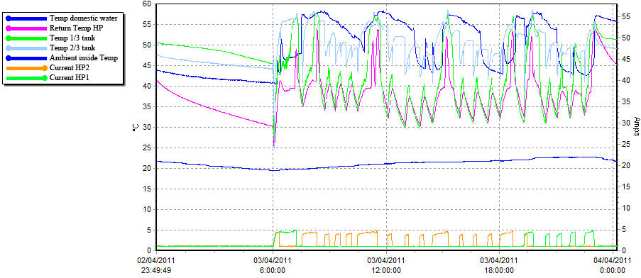
Data heat pump in the 3rd case study in Ballencrief 08/03/2011
The curves red and black correspond to the temperatures of the water flow coming from the Heat Pumps. For the heat pump 1 (HP1), the sensor was located in the tank. Thus, when the heat pump is not operating, the temperature measured is close to the temperature of the tank. For the heat pump 2, the sensor is far from the tank. When it is not working the temperature normally decreases because of the heat losses with the environment.
The return temperature to the heat pumps is quite high considering the quite mild temperature, from 35 to 40C during normal operation. It is a bit higher in general than the return temperature from the radiators. The starts and stops of the compressor are also in this case quite frequent, as well as the sterilisation cycle.
Data energy demand in the 3rd case study in Ballencrief 08/03/2011
In term of energy demand there is quite a lot of domestic hot water demand. The blue curve corresponds to the temperature of the pipe for the domestic hot water. When there is not hot water consumption, the temperature decreases because of the heat losses in the environment.
The radiators are also used the whole day. However the temperatures are quite mild since the outside temperature is quite low. There are quite a lot of temperatures fluctuations according to the operation of the heat pumps.
Data tank performances in the 3rd case study in Ballencrief 08/03/2011
With this tank, the stratification of the temperatures during the system operation is always conserved. The hot water coming from the heat pumps is indeed released at the top of the tank. However the temperatures at the bottom of the tank are fluctuating quickly according to the actual operation of the heat pumps. The water for the radiator is mainly taken at the bottom of the tank.
The heating system enables to increase the temperature in the house during the whole day. The set point is quite high. At 23C of ambient temperature inside the House, the heating system is still working.