Housing Loads
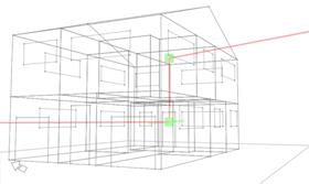
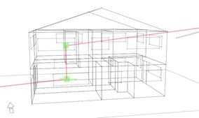
In order to establish load profiles for the electrification of housing for heating, small power and lighting loads, a dynamic simulation model using the IES software package was undertaken. Figures 1 and 2 illustrate different views of the model. In order to create a realistic load profile of a scenario that would be typical of a house in today’s world, specific assumptions were made that were supported by the literature review, and are as follows;
Figure 1 – 1st Isometric View of Model Figure 2 – 2nd Isometric View of Model
Occupancy Profiles
Occupancy profiles can come in many shapes and sizes, but as part of this project the decomposition of the society was split into two main profiles and this was considered important as part of the considerations of what would be typical of the UK domestic housing sector. These reflections are as follows;
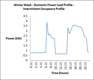
- Intermittent Occupancy (figure 3).
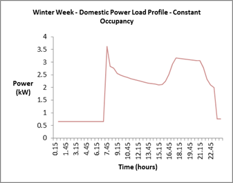
- Constant (figure 4).
The intermittent occupancy profile was representative of a typical working class family, which characterises quite a significant proportion of houses within the UK. In this case the demand for heating, hot water, lighting and small power during the day would be almost negligible due to the highly intermittent nature of this occupancy pattern.
On the other hand, the constant occupancy profile would be representative of a parent with young kids or an unemployed or retired person. In this instance the demand for heating, hot water, lighting and small power might have been more constant throughout the day with perhaps less spikes occurring at peak times in the morning and evening.
By creating these two profiles it was valid to run different simulations based on these occupancy patterns to create load profiles that were representative of domestic housing within the UK.
Climate Data
For the purposes of this modelling exercise the annual climate data was extracted from the ASHRAE database, in IES, for a Glasgow location and the simulation was carried out on an annual basis.
Geometry Attribution
There are many different shapes and sizes associated with a typical UK house and so for the purposes of this exercise assumptions were made on the average size. In order to do this, as part of the literature review, it was defined that the average size of a UK domestic house was about 91m2 and typically in the form of a two storey house (Department for Communities and Local Government, 2010) (Ministry of Infrastructure of the Italian Republic). The model was based on this average figure and a breakdown of those rooms is shown in the tables 1 and 2 below. Figures 5 and 6 illustrate the isometric views of the ground and first view of the house.
Category |
Description |
Data source |
U value (W/m2K ) |
Thickness (mm) |
Roof |
flat roof |
Generic |
0.18 |
317 |
Internal Partition |
13mm pll 105mm bri 13mm pll |
Generic |
1.9948 |
30.7 |
Internal Ceiling/Floor |
Carpeted 100mm reinforced-concrete ceiling |
Generic |
1.2498 |
615 |
Ground/Exposed Floor |
standard floor construction (2010 regs) |
Generic |
0.22 |
1348.7 |
External Window |
low-e double glazing (6mm+6mm) (2010 regs) |
Generic |
1.8 |
24 |
External Wall |
standard wall construction (2010 regs) |
Generic |
0.2599 |
208.9 |
Door |
wooden door |
Generic |
2.1997 |
37 |
Table 1- House Details
Room ID |
Room Name |
Volume (m³) |
Floor Area (m²) |
ROOM0005 |
BEDROOM 1 |
24 |
8 |
ROOM0009 |
BEDROOM 2 |
31.5 |
10.5 |
ROOM0006 |
BEDROOM 3 |
24 |
8 |
ROOM0007 |
BEDROOM 4 |
25.5 |
8.5 |
ROOM0011 |
CIRCULATION |
27 |
9 |
ROOM0001 |
DINING RM |
21 |
7 |
ROOM0010 |
ENSUITE |
27 |
9 |
ROOM0002 |
HALLWAY |
24 |
8 |
ROOM0003 |
KITCHEN |
30 |
10 |
ROOM0000 |
LIVING ROOM |
27 |
9 |
ROOM0004 |
WC |
12 |
4 |
TOTAL |
|
273 |
91 |
Table 2- Room attribution
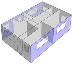
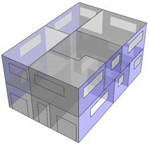
Figure 5 - Isometric View of Ground Floor Figure 6 – Isometric View of First & Ground Floor
Constructional Attribution
In order to model a house that was typical of today’s society, the following parameters were used in the model for fabric and glazing data, based on the most recent building regulation standards (HM Government). Details of which can be seen in the table 3 below;;
Limiting Fabric Parameter Inputs (HM Government) |
|
Roof |
0.20 W/(mK) |
Wall |
0.30 W/( m2K) |
Floor |
0.25 W/( m2K) |
Party Wall |
0.20 W/( m2K) |
Windows, Roof windows, |
2.00 W/( m2K) |
Air Permeability |
10m3/(hm2) at 50 Pa |
Table 3- Fabric Parameters
Systems Attribution
In order to address the energy demands within the building such as lighting and small power, references to industry standards and manufacturers data were applied. Typical lighting levels were obtained from the following table 4, and these levels were carefully added using a standard lighting profile in the winter and summer months in the IES simulation model (CIBSE, 2002).
Area |
Illuminance (lux) |
Lounge |
100-300 |
Kitchen |
150-300 |
Bedrooms |
150 |
Bathroom |
100 |
Table 4- Illuminance
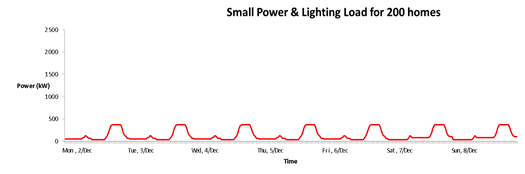
Figure 7- Small Power & Lighting Load
For the baseline simulation 0, the gas fired boiler system was modelled and included a system efficiency of 0.89 as this would be typical of a conventional boiler system in a house, that represented the ‘now’ scenario illustrated in figure 7. When switching from the gas fired boiler system to heat pump system, a Coefficient of Performance (CoP) of three was used as this was the typical seasonal average efficiency that most heat pump manufacturers claimed to achieve. Then upon switching to an electric heating system, a 100 litre hot water electric storage tank was also included to increase the progressive levels of electrification..
Calibration of Results
At the beginning of the project, in order to obtain the heating, small power and lighting loads it was envisaged that this data could be taken from the real world, e.g. existing operational buildings. This proved difficult however, as the information that was obtained only gave snippets of information. So in order to address the building demand loads a dynamic simulation was carried out for each scenario. The information that was produced was then calibrated against the snippets of information for the base case. Due to the limited information on future simulations the calibration only took account of the base case and further scenario simulations worked from this calibration.