Solution techniques
The solution techniques used in ESP-r are described in a 2007 paper by Clarke, Kelly and Tang:
...An ESP-r model may comprise many different and diverse constituent parts of varying levels of detail (e.g. constructions, moisture flow, electrical networks, air flow networks etc). However, as each part is based on the same finite volume considerations, when connected together, they form a consistent mathematical description of the building, no matter the level of detail adopted. ...
Within ESP-r the set of equations associated with each technical domain are solved by optimised methods that are targeted to the specific nature of the equations – be they sparse, linear, non-linear, mathematically stiff and so on. The important point is that no attempt is made to concurrently solve the whole system equations. Instead, the domain equations are solved independently under the control of a supervisory routine that respects the physical couplings between domains (e.g. the bi-directional coupling between air and heat flow). ...
The integrated solution of all domains therefore requires the co-ordinated application of the domain solvers applicable to the particular model being used.
heat transfer within thermal zones
The 2007 paper also links the solution process to energy balances:
The conductive, convective and radiation exchanges associated with a building’s constructions are established as a set of energy balance equations and a direct solution method applied. The approach is based on a semi-implicit scheme, which is second-order time accurate, unconditionally stable for all space and time steps and allows time dependent and/or state variable dependent boundary conditions and coefficients. Iteration is employed for the case of non-linearity where system parameters (e.g. heat transfer coefficients) depend on state variables (e.g. temperature). An optimised numerical technique is employed to solve the system equations simultaneously, while keeping the required computation to a minimum.
Further details are found here.
network air/water flows within the model
The paper also provides an overview of solution of mass balance within networks of air or water:
The approach is based on the solution of the steady-state, one dimensional, Navier-Stokes equation assuming mass conservation and incompressible flow. The result is a set of non-linear equations representing the conservation of mass as a function of pressure difference across flow restrictions.
And further information can be found here.
heat and mass flows in plant components
As with the zones that make up the building model, the control volume technique is also used to derive the equation sets describing a building’s plant network. Within ESP-r the plant network consists of a coupled group of plant component models, each described by one or more control volumes. The author of the component can thus include considerable internal detail. Indeed one finds both a simple (two node) and a complex (8 node) radiator definitions. More information is found here.
electrical power distribution
To facilitate the study of renewable energy systems integration an electrical power distribution data model and solver were incorporated into ESP-r in ~1994 and these have evolved over time to support studies of battery and fuel cell and electrical vehicles. Further discussion is found here.
CFD domain
Again from the 2007 paper:
Flow inside a room is characterised by a set of time-averaged conservation equations for the three spatial velocities (U, V, W), temperature θ and concentration C. For turbulent flows two additional equations are added, for turbulence intensity (k) and its rate of dissipation (ε). As with the building thermal domain, these conservation equations are discretised by the finite volume method. ...
Because these equations are strongly coupled and highly non-linear, they are solved iteratively for a given set of boundary conditions. The SIMPLEC method is employed in which the pressure of each cell is linked to the velocities connecting with surrounding cells in a manner that conserves continuity.
Further discussion is found here..
Solver sequencing
Again from the 2007 paper:
...the solution process employed within ESP-r links the various technical domain solution methods (direct or iterative) together through a flexible process of iterative ‘handshaking’ at key linkage points. This handshaking involves solving the subsystem equation sets separately, based on previous time step values of the coupled variables and then iterating to a solution.
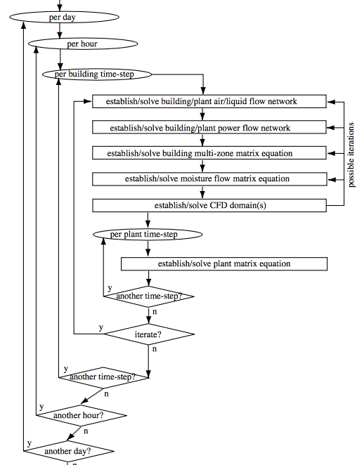
[with reference to the figure below]
At each building-side time step and for a given climate boundary condition, the air/liquid flow networks corresponding to the building and plant are established, control considerations imposed and the equations solved. Solution of these networks gives the air and working fluid flow rates throughout the building and within the plant system respectively. The electrical power flow network representing building-side entities (e.g. lighting, small power, photovoltaic facades etc) and plant components (e.g. fans, pumps, CHP plant etc) is established, constrained by control action and the equations solved. The facility may be used to impose demand side actions on load consuming systems. (This network model and the preceding one for air/liquid flow may also be invoked at higher frequency from within the HVAC solution loop.)
The building-side, multi-zone matrix equation is then established using the latest estimates of the fluid/power flows and plant induced flux injections/extractions. Equation solution is achieved as described previously to obtain the building's temperatures and heat flows. Using the newly computed intra-construction temperatures, the construction moisture flow matrix equation is established and solved. This gives the moisture distribution within the building fabric. Using the building temperatures and air flow rates as boundary conditions, the CFD model is established and solved. This gives the intra-zone distribution of temperature, velocity, pressure and contaminants. The building temperatures and air/liquid flow rates are then used, along with relevant control loops, to establish and solve the plant heat and mass flow matrix equations. Solution of these equations gives the plant temperatures and flow rates.
Free floating zones supported
Rooms not currently subjected to environmental controls free float. The air temperature derives from the zone energy balance. Some control definitions which include a dead-band also result in free floating conditions if the current sensed condition is within the dead band.
Assessment frequency
The timesteps in each domain can be set by the user subject to a few constraints imposed by the data structure (for example some data-holding arrays in the results recovery module are sized to allow a one minute resolution). Currently the timestep ranges for each domain are:
Rewind control
Some control laws such as optimal start and optimal stop can invoke a rewind control. The assessment saves its state and jumps back to the start of the day to see if an alternative approach yields better results. This is a rarely used facility and occasionally the results recovery reporting may time-shift.
Implicit or Explicit solution
The zone solver accepts user directives to alter the technique from fully implicit to fully explicit although the default is simi-implicit.
Convergence criteria
The ESP-r simulator is normally stable whatever the nature of the building or system being assessed. Most users will never touch the convergence criteria. For experts or those who are pushing the boundaries of the virtual physics there are a number of options (but they are password protected):
Back to top | Back to Welcome page