Zone solvers

Overview

The following is taken from a 2007 paper by Clarke, Kelly and Tang:

The building is broken down into many small control volumes to which the conservation of mass, energy, momentum, species and so on can be applied. While the characteristics of control volumes can vary – homogeneous or non-homogeneous, solid or fluid, size and shape – the conservation principle can be uniformly applied as appropriate. These control volumes may be used to model a building in whole or part while including the multiplicity of interacting physical processes. Typically, a building model will comprise many thousands of control volumes, each assigned one or more conservation equation depending on the physical processes impacting on the region.
Control volume equations represent the fundamental physical processes occurring within the building, e.g. heat conduction and storage, air and moisture movement, radiation exchange, electricity flow etc. Within ESP-r related sets of equations are grouped and each group processed by a tailored solver that is optimised for the equation set type. Solution of the equation sets, with real climate data and user defined control objectives as boundary conditions, gives rise to a detailed and integrated view of performance evolution over time.
A particular attraction of the control volume approach is that the same physical process can be modelled at different levels of detail. For example, the air within a zone may initially be modelled as a single control volume, which corresponds to the assumption that the air is well mixed. At a later stage this single control volume can be replaced by multiple control volumes to facilitate network air flow or enhanced resolution computational fluid dynamics.

Zone and surface heat flow paths

Energy balances at zone air nodes and at the inside and outside face of each surface are resolved at each timestep. The heat flow paths within the zone energy balance are discussed here. The heat flow paths at the inside face and outside (other) face of constructions are discussed here.

Contributing to the solution of each flow path are so-called sub-systems e.g. subroutines which resolve a specific issue such as surface-to-surface radiant heat transfer, solar insolation distribution, the establishment of heat transfer coefficients and the like. The methods used are often described within the source code as well as in the Clarke Book Energy Simulation in Building Design.

One of the few steady state treatments within the energy balance is used for linear thermal bridges. This is a pragmatic approach when a full 2D or 3D conduction grid has not been imposed on the solution.

Environmental control actions can be applied (e.g. heat injected or extracted):

at a layer within a construction in a zone e.g. an embedded heating pipe

at the zone air node e.g. a convective injection

a mixed convective radiant injection to the zone air node and to surfaces in the zone (apportioned by area and emissivity).

Long wave radiation

Longwave radiation exchanges between surfaces in zones is handled separately from surface convection and is based on a grey-body approach with the option to calculate explicit surface-to-surface viewfactors. For surfaces facing ambient conditions these follow model level conventions of views to the sky, ground and other buildings. More information is available here.

Convection

ESP-r offers a range of facilities to evaluate convection at surfaces as well as to specify specific convection regimes or heat transfer coefficients. At the extreme, a coupled CFD assessment can be used to derive heat transfer coefficients at each timestep based on the flow field. More information is available here.

Moisture transfer

The solution of mass flow balances includes bookkeepping for the transport of moisture and the tracking of humidity within zones. Casual gains which have a latent component also take part in this process as do ideal environmental controls which include humidification or dehumidification. The mass flow solver also includes basic moisture tracking.
This can be extended by treating moisture as a contaminate source and specifying the adsorption properties of constructions in rooms. This is often problematic as such attributes may not be readily available and specialist tests are needed to establish the relevant parameters. More information on the numerical approach is available here.

Range of constructions and materials

The underlying computational approach supports most mixes of materials and material thicknesses. ESP-r is particularly adept at handling traditional mass constructions and readily accepts PCM definitions as well as materials with electrical or electrochromic properties. There are a few caveats: single layers in constructions should generally be less than 250mm and greater than 0.5mm; thin metal layers against insulation may require shorter timesteps to avoid numerical stress.

Simulation startup

One user directive is the pre-simulation period, a value is suggested based on the time constants of the constructions used in the model. Weather data is taken from a period prior to the actual assessment - e.g. a 5 day warmup for an assessment beginning on the 6th of May would start on the 1st of may. No performance data is recorded during the startup period.

Simulation frequency

The initial default is a 15 minute timestep for the zone solver and this can be adjusted from one minute to one hour. Systems solve at a multiple of the zone timestep. This multiple can be adjusted from one to ~one hundred. With large models at short timesteps the results files many grow to scores of GB and this can also extend the resources needed for data-mining.

Dynamic changes in models

The simulator normally scans the model at the start of the assessment and only adapts the form and composition of the model if specific directives are in place. An example would be switching the composition of surfaces (to mimic shutters).

A rarely used facility allows the orientation and or the location of the model to be adjusted as the assessment progresses to mimic a vehicle or ship.

Model complexity

Model complexity is limited both by the skills levels of the user as well as the compiled-in limits of the software. ESP-r can be compiled for low-resource computers and alternative header files exist (and can be further edited and ESP-r modules re-compiled). Three typical compile-complexity ranges are:

low resource deployments - 32 zones, 80 surfaces/zone, 2000 model surfaces, 40 obstructions per zone, 12 layers per construction, 32 controls, 40 flow nodes, 100 flow connections, CFD grid 18x18x18

standard deployments - 82 zones, 80 surfaces/zone, 3000 model surfaces, 120 obstructions per zone, 16 layers per construction, 82 controls, 80 flow nodes, 200 flow connections, CFD grid 32x32x32

workstation deployments - 82 zones, 96 surfaces/zone, 4000 model surfaces, 180 obstructions per zone, 16 layers per construction, 82 controls, 86 flow nodes, 200 flow connections, CFD grid 32x32x32

ESP-r is a general purpose tool with an extensive data model which allows opinionated users to create models fit for purpose as well as allowing experts to craft bespoke models. Allowing the user to be in charge of what gets included in the virtual world implies a learning curve and it rewards those who have a good background in building physics. This said, some simulation tasks are straightforward and ESP-r has been used for both undergraduate and graduate teaching as well as consulting. As a rough guide novices and experienced users who invest time in gaining skills might expect the following:

novices should be able to work with models with a dozen zones, e.g. residential or small office projects. They should be able to work with ideal controls and simple flow networks would not be well equipped for using system components or CFD assessments.

experienced users should be able to push to the nominal limits of the tool but will be most productive with models short of the absolute limits.

Computational resources

ESP-r runs on a range of computational platforms and operating systems from single-board ARM computers such as the Raspberry Pi to compute servers. A list can be found here.

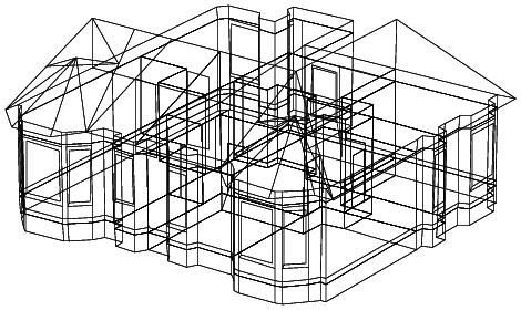
An example of the computational resources needed for an annual assessment at a 15 minute timestep of the model shown in the figure below. The model has 13 thermal zones, 432 surfaces, 12 ideal controls enabling WCH, high mass constructions (up to 700mm of stone in facade).

In the list below are run-times for ESP-r compiled with no optimisation and highly optimised directives:

Raspberry Pi (orig) 19425(s) 7845(s)

Raspberry Pi 3 8400(s) 2150(s)

Lenovo T61 laptop 1015(s) 275(s)

Apple Macbook Pro (mid 2012) 682(s) 182(s)

Dell 780 720(s) 188(s)

Dell 7010 448(s) 139(s)

Optional directives

ESP-r works on a functionality follows description approach. The user decides what constitutes a zone and what is included as well as the level of detail in the form and composition. The addition of new information often will trigger an additional computational domain to be included in the assessment. For example initial scheduled air flows can be superseded by a flow network. Beyond this, there is a long list of optional directives to either enhance the resolution of the assessment - e.g. computed shading and insolation, computed surface-to-surface view factors, sensor bodies within the model and convective regime directives. The simulation engine then responds to the included descriptive entities and assessment directives. The simulator does, however contain a number of simulation toggles that experts can use to disable or enable specific functionality.