The Tool
This page is designed to highlight how the tool was created. To directly see a tutorial of our tool (Far Offshore Wind Interactive Tool - FOWIT), Click Here.
Both, preventive and corrective maintenance, were considered in our analysis. Inputs for both types of maintenances could vary depending on the particular wind farm. Thus corrective and preventive inputs could be easily modified once the necessary data is provided.
Preventive Maintenance
The aim of the preventive maintenance is to determine if a major work has to be carried out. Thus preventive maintenance will include activities like routine inspections or checks (of particular components). Some of the modern preventive methods are implementing new condition monitoring technologies [14]. If there is a need to perform a considerable amount of work on a wind turbine, it means that a turbine could be shut down. Hence the main idea is to avoid shutting down wind turbines and also to make sure that the amount of corrective activities is minimized. A wind turbine would undergo a full servicing every six months [15].
Corrective Maintenance
Corrective Maintenance is performed as a reaction to issues with wind turbine’s components, which could be caused by several different things, e.g.
- Aging of a component
- Faulty design
- Operational factors, etc.
Technicians become aware that it is necessary to go ahead with corrective maintenance during an inspection of a wind turbine or when the turbine shuts down due to a fault [15].
Common Inputs
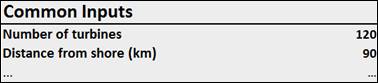
The common parameters required to perform the analysis are allocated in this section. A brief description of each parameter is provided below.
- Number of turbines: Number of turbines in the wind farm.
- Distance from shore (km): The distance from the closest port to the wind farm, maybe the distance from shore is less, but since it is considered for travel distance issues, it should be from the port.
- Capacity of turbines (MW): The rated power per turbine.
- Work shift hours per day (h): The period when technicians will work per day. For instance, a usual work shift is 12 hours, e.g. from 6 am to 6 pm.
- Number of technicians per CTV: How many technicians could be carried by one CTV.
- Speed (kn): The speed of crew transfer vessel, it will be used for calculating travel times. Standard value would be 20 knots.
- Cost of personnel (£): Cost of each technician per hour for doing maintenance operations. This value would be considered as the cost per hour of permanent technicians rather than temporary technicians’ cost per hour. Standard value would be £ 40.
- Lifetime (yr): Number of years of operation considered in the analysis. Standard value would be 15 years.
- Operators, Sharing (-): It is assumed that one wind farm with previously defined parameters will be considering a charter of purchase of a vessel. This parameter defines the operator sharing percentage of the vessel employed as offshore accommodation. Therefore, the cost of the vessels will be taken into account according to this percentage. In case of spot market, the option of sharing will not be considered due to the fact that by hiring the vessels daily there is no possibility to share it between different operators.
- Discount factor: It is considered the money is more valuable at a present time rather than in the future. Therefore, it is better to include costs later rather than sooner. That allows you to make investments and gain more benefits in the meantime. Thus in order to highlight this aspect of financial analysis, a discount factor is included, discounting the cost within the analysis in annual basis. In terms of purchasing a vessel, this parameter is very important because a high capital cost is paid at the beginning.
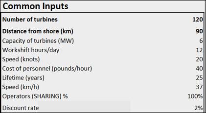
Figure 5: Common Inputs
Preventive Maintenance Inputs
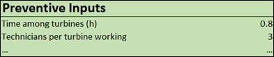
- Time among turbines (h): As a CTV is able to transport a certain number of technicians (for instance 12), one CTV could be employed to do maintenance among several turbines. This number involves accessing a wind turbine and travel time between one turbine to another. Here, the number represented by time among turbines describes time between two turbines.
- Technicians per turbine working (-): Number of technicians required per turbine to perform maintenance operations.
- Turbines/CTV: This parameter represents how many turbines can be maintained using one CTV. Normally, it will be the number of technicians per CTV divided by the number of turbines that a CTV can do maintenance at the same time (turbines/CTV).
- Time required for doing preventive maintenance per turbine and per year (hr): Each turbine requires a list of operations that should be performed each year. This parameter represents how many hours of work are necessary per turbine during one year. For this part of analysis the regular preventive maintenance (annual) is only considered. There are other maintenance revisions that are not considered, for example long-term revision.
- Days estimated for preventive maintenance (day): Operators usually perform preventive maintenance once per year during a scheduled period of time (time-based maintenance). This value represents how many days that preventive operations will take. As it is an estimation, a range will be more appropriate rather than a value, therefore, in the analysis both an upper limit and a lower limit will be considered:
- Upper limit of days estimated
- Lower limit of days estimated
- Number of CTV (-): The number of CTV employed for carrying out preventive maintenance operations. This number can be introduced manually, however, depending on the number of CTV, the days required would be different as the days estimated for doing preventive maintenance. In that case a VBA code has been created to calculate how many CTV are required for the analysis. Thus, this input will usually be automatically calculated. The VBA code will be explained later.
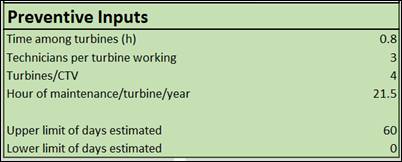
Figure 6: Preventive Inputs
Preventive Maintenance Intermediate Outputs
- Time available employing per CTV (h): As mentioned before, each CTV will go to more than one turbine each day in order to perform maintenance operations. Furthermore each vessel can handle a number of technicians, and those technicians are contracted to work certain amount of hours per day. Hence, the time available should take into account that technicians will only be working the work shift hours including travel times, repair time and transfer time between wind turbine So the total time available will be the work shift hours multiplied by the days of maintenance that year.

*For example, assume that each day one CTV that carries 12 technicians. The total time available that day will be 12 hours, including travel and maintenance time. Therefore if the preventive maintenance takes 10 days, the total time available using that CTV will be (12 * 10 = 120), 120 hours.
- Travel time from shore (h): Time required for travelling from shore to the wind farm. Here the speed of vessel and distance are taken into account

*This number will vary depending on the solution chosen, if a CTV (no offshore accommodation) is considered, then it will be necessary to travel from shore to the wind farm every day. Nevertheless, when offshore accommodation option is chosen, it is not necessary to travel from shore to the wind farm so often.
- Time among turbines per day (h): This number represents how many hours per day are considered to travel among wind turbines per CTV. As mentioned before, each CTV will go to more than one turbine per day. Thus it will be necessary to take into account the turbines per CTV per day. This number changes when considering different solutions
- Without offshore accommodation: CTV travels from shore to the first turbine. Afterwards the CTV will go to other turbines and at the end CTV returns from the last turbine to shore. Since the time from returning to the shore is already considered (travel time from shore), only the time between the first turbine and the last turbine should be considered. For example: if each CTV goes to 4 turbines per day, then this time will include the time between the first and second turbine, second and third turbine and finally third and fourth turbine, i.e. three transfers in total.

- Offshore accommodation: If offshore accommodation is considered, the travel time from the accommodation to the first turbine and the returning travel time should also be considered, along with the time between the turbines. For instance: if each CTV go to 4 turbines per day, then this time will include time between offshore accommodation and first turbine, first and second turbine, second and third turbine, third and fourth turbine, and finally fourth turbine and offshore accommodation, five processes in total.

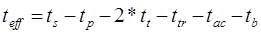
- Effective time per day per CTV (h): This number represent the actual time when maintenance could be performed in the turbines per day.
teffective = tavail - ttravel + tamongturbines
- Days required to accomplish maintenance per operation: As mentioned before each turbine will require a maintenance time per year (time required for doing preventive maintenance per turbine and per year (hr)). Since the work shift time each day should take into account travel time and effective time, maybe in one day the preventive maintenance tasks could not be accomplished. This number represents how many days are required per operation (which means per CTV), in order to accomplish the specified preventive maintenance time.

*Example: one CTV will go to 4 wind turbines, and each day the time effective per day is 5 hours. Let’s say that each wind turbine required 20 hours of preventive tasks per years. Therefore, the time needed to accomplish preventive tasks will be (20/4 = 5) 5 days. It means that in 5 days using one CTV, preventive tasks for 4 wind turbines will be accomplished.
- Days required per year: This number represents how many days are required for accomplishing all the turbines maintenance operations each year. It will take into account the previously mentioned assumptions, each operation using one CTV will go to different wind turbines each year.

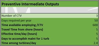
Figure 7: Preventive Intermediate Outputs
- Explanation of VBA code (Calculating the number of CTV):
As showed in the above formula, the time required each year depends on the number of CTV employed. Therefore, if more CTV are used, the preventive task will be accomplished faster (less required days). When calculations are performed, it is difficult to choose how many CTV should be considered. Hence, a VBA code has been created in order to calculate how many CTV are needed. As mentioned before, operators normally establish a number of days in order to perform preventive tasks considering time-based preventive maintenance. Thus, CTV number will be calculated according to the limits specified in the inputs.
If the days required for performing preventing tasks exceeds the upper limit, more CTV will be added, and if the days required are less than the lower limit, CTV will be subtracted.
Preventive Maintenance Outputs
- The main output of this analysis will be the total cost of the personnel during preventive tasks each year. As the number of days for doing preventive maintenance each year (Days required per year) and the number of CTV (Number of CTV) are already calculated in the intermediate outputs, it is only necessary to take into account the number of technicians per CTV (Number of technicians per CTV), work shift hours per day (Work shift hours per day), and the cost of technician per hour (Cost of personnel) in order to calculate the total personnel cost.


Figure 8: Preventive Maintenance Outputs
Corrective Maintenance Inputs
The failures that appear in a wind turbine and require corrective maintenance tasks are divided into five main categories as in Table 1.
Table 1: Categories of corrective maintenance tasks [22]
| Category |
Description |
Repair actions required (h) |
Logistics time (h) |
| A |
Repair, cleaning no replacements |
3 |
0 |
| B |
Repair Cleaning replacement of consumable |
3 |
8 |
| C |
Replacement small parts |
10 |
48 |
| D |
Replacement large parts > 50 tonnes |
96 |
160 |
| E |
Replacement rotor, nacelle, yaw, main bearing < 300 tonnes |
96 |
500 |
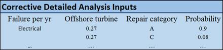
The repair hours and the logistics time that each one of the tasks requires are also indicated in Table 1. The last one consists of the procurement of the consumables or spare parts, or the deployment (chartering, organising crew) of special application vessels (jack-up). The failures that occur in an offshore wind turbine are analysed by categorising them according to the above methodology, and probabilities for each case are given as in Table 2
[22]. With this way, the impact of each category of failure in the downtimes can be derived more accurately, since each one of them requires different amount of hours to perform the necessary repair.
Table 2: Failure rate of offshore turbine [22]
|
Failure per year for
offshore turbine |
Repair category |
Probability |
Category of maintenance required |
fi (Failure rate per year) |
| Electrical 0.27 |
A |
0.9 |
A |
1.0515 |
| D |
0.02 |
B |
0.014 |
| E |
0.08 |
C |
0.0117 |
| control unit 0.21 |
A |
0.5 |
D |
0.1107 |
| E |
0.5 |
E |
0.3521 |
| Inverter 0.2 |
A |
0.9 |
Total |
1.54 |
| E |
0.1 |
| Yaw system 0.2
| A |
0.65 |
| E |
0.34 |
| C |
0.01 |
| Brakes
0.05 |
A |
0.8 |
| E |
0.2 |
| Gearbox 0.25 |
A |
0.85 |
| E |
0.05 |
| D |
0.1 |
| Generator 0.13 |
A |
0.5 |
| D |
0.3 |
| E |
0.2 |
| Pitch 0.15 |
A |
0.5 |
| E |
0.5 |
| Blade 0.07 |
B |
0.2 |
| C |
0.01 |
| D |
0.59 |
| E |
0.2 |
| Shaft and bearing 0.01 |
A |
0.1 |
| C |
0.9 |
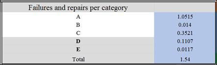
Figure 9: Corrective Maintenance Categories
Corrective Maintenance Outputs: Downtime or Outage Cost
Introduction
The main purpose of this modelling approach is to calculate downtimes for 3 different cases of O&M: the traditional method of travelling from shore using CTV, the jack-up vessel and the mothership. The cost of the downtimes in each case is derived in terms of losses of power production, and the contribution of each alternative in O&M cost reduction is highlighted.
CTV from harbour
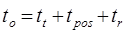
The total downtimes from failures of each category are presented in Table 3, where the tr and tl variables are the ones shown in Table 1. The to Operation time is calculated as follows:
Categories A, B, and C


Where:
| tp |
Preparation time (h) |
| tt |
Travel time (h) |
| ttr |
Transfer time (h) |
| teff |
Effective time (h) |
| ts |
Work shift (h) |
| tac |
Acclimatisation due to long travel time (h) |
| tb |
Break (h) |
| D |
Distance to shore (m) |
| S |
Speed of vessel (km/h) |
And div represents the integer division. In these categories of small components replacements the time for the operation hours spent incurs from the transfer mission and the repair. It is considered that if a repair cannot be performed in one working shift, then the turbine remains inoperative as many days as necessary to complete the task. The day that the operation will end takes into account only the travel to turbine and not the travel back to harbour, due to the fact that the operation is restored after the technicians leave the site. Preparation, travel, transfer, acclimatisation and break times are constants acting as inputs of the model.
Category D
In this category a crane ship is chosen and the operation time is calculated from:

Where the travel time is different due to the slower speed of the vessel, and the repair time which includes putting cranes and spare parts to platform, hosting and mounting intermediate crane and 50 tonnes crane to nacelle, let down the failed part and mounting of new part.
Category E
In this case a jack-up vessel is used and the time spent in operation is calculated as follows:
Where tpos is the time spent in the positioning of jack-up.
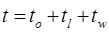
Adding the necessary logistics time, and the weather delay in each operating time the total downtime t of each category can be derived.
It is noted that the logistics of the jack-up comprise of organising crew, chartering the jack-up (which can take up to weeks due to low supply of these vessels) and finding spare part.
Table 3: Downtimes for the case of CTV from shore [22]
| Category |
Travel time (h) |
Repair time (h) |
Operation time(h) |
Logistics time (h) |
Weather delay (h) |
Total downtime (h) |
| Equation |
tt |
tr |
to |
tl |
tw |
t |
| A |
4.1 |
3 |
57.2 |
0 |
70 |
127.2 |
| B |
4.1 |
3 |
57.2 |
8 |
70 |
135.2 |
| C |
4.1 |
10 |
184.2 |
48 |
70 |
302.2 |
| D |
10.0 |
96 |
106.0 |
160 |
70 |
336.0 |
| E |
12.0 |
96 |
108.0 |
500 |
70 |
678.0 |
Jack-up vessel for O&M
In this case it is considered that the technicians reside in the platform of the vessel, therefore the travel time is zero. Assuming that all the available spare parts are stored in the platform, the logistics time is also considered to be zero. The corresponding downtimes when using jack-up for O&M are indicated in Table 4.
Table 4: Downtimes for the case of jack-up vessel for O&M [22]
| Category |
Travel time (h) |
Repair time (h) |
Operation time(h) |
Logistics time (h) |
Weather delay (h) |
Total downtime (h) |
| Equation |
tt |
tr |
to |
tl |
tw |
t |
| A |
0 |
3 |
4.6 |
0 |
70 |
74.6 |
| B |
0 |
3 |
4.6 |
8 |
70 |
82.6 |
| C |
0 |
10 |
11.6 |
48 |
70 |
129.6 |
| D |
0 |
96 |
97.6 |
0 |
70 |
167.6 |
| E |
0 |
96 |
97.6 |
0 |
70 |
167.6 |
Mothership
For the failures that require small replacements, the mothership offers the same advantage as a jack-up, as technicians do not have to travel from shore, which will result in zero travel time. However, in the replacement of large components (D, E) the tasks of chartering crane ship and jack-up vessel have to be performed as in the case of CTV. The main advantage of this solution is that the mothership can operate in higher wave heights reducing the delay due to bad weather conditions significantly (Table 5).
Table 5 : Downtimes for the case of mothership for O&M [22]
| Category |
Travel time (h) |
Repair time (h) |
Operation time(h) |
Logistics time (h) |
Weather delay (h) |
Total downtime (h) |
| Equation |
tt |
tr |
to |
tl |
tw |
t |
| A |
0 |
3 |
4.6 |
0 |
20 |
24.6 |
| B |
0 |
3 |
4.6 |
8 |
20 |
32.6 |
| C |
0 |
10 |
11.6 |
48 |
20 |
79.6 |
| D |
6.7 |
96 |
102.7 |
160 |
20 |
282.7 |
| E |
9.0 |
96 |
105.0 |
500 |
20 |
625.0 |
Then the downtimes for each category in each solution can be derived. Hence the total downtimes for each option of O&M can be found. This is calculated from:
Where:
is the indicator of the category of the failure.
Power Production losses
Having calculated the downtimes caused in each case of different O&M solution, the cost incurred from the power production losses of the wind farm can be calculated, as follows:

Where:
| CAP |
Capacity of wind turbine (KW) |
| Nt |
Number of turbines |
| CP |
Capacity factor |
| Cel |
Electricity price (£/KWh) |
Therefore, the critical inputs and output of the modelling approach are summarised in Table 6.
Table 6: Inputs and output of the cost modelling
| Inputs |
Capacity of turbine |
Number of turbines |
Capacity factor |
Electricity price |
Distance from shore |
| Output |
Costs of downtimes due to failures from power production losses for each O&M scenario |
Change of failure rates with time
During the total operation lifecycle, the performance and reliability of the offshore wind turbines is a subject to vary. The pattern that expresses the behaviour of the wind turbine failures intensity (throughout the lifetime of operation) resembles the one of a bathtub curve (Figure 5) [23]. This distribution is produced using a special case of Poisson process suitable for repairable equipment, and it has a density function as follows:
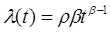
Where:
| β |
Shape parameter that indicates the trend |
| ρ |
Units per year |
| λ |
Failures per turbine per year |
>
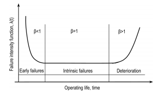
Figure 10: Change in failure rates of the wind turbines through time, [23]
Figure 10 presents 3 stages of a lifecycle of a wind turbine and related failure intensity. In the early operating life, β<1 period, a turbine may experience problems regarding design improvements and alterations on field. During the β=1 period, the tear and wear has appeared and the equipment is less likely to need modifications. At the end of the lifetime, β>1 period, turbines are aging which leads to degradation of the materials. In [23] the time t is expressed as total time on test and represents the summative quantity of all running hours of all turbines until a failure appears. In the excel tool the time t has the meaning of calendar time and takes the discrete values of years of operation. An example of a category of failures calculated throughout 25-year lifecycle is demonstrated in Figure 11 below.
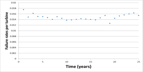
Figure 11: Failure rates through time for category B (repair, cleaning, and replacement of consumables), [23]
Cost of vessels. Inputs.
Three main solutions considered are no offshore accommodation, mothership or jack-up. In addition, three different markets are examined for each type of vessel:
- Spot market: The vessel is hired on a daily basis depending on the days required for doing preventive maintenance tasks.
- One year charter: The vessel is chartered for one year, thus it is available when required all the days within a year.
- Purchase: The vessel is purchased, a capital cost must be considered at the beginning, after an operational cost should be considered for each year of operation.
Furthermore, CTV are employed in each solution. In terms of no offshore accommodation CTV are the main vessel type. However, when considering offshore accommodation (mothership or jack-up), CTV are needed to perform the preventive operations (travelling from the offshore accommodation vessel to the selected turbines). In conclusion, there are 21 potential solutions considering both the vessel type and financial option.


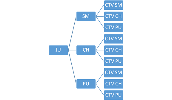
* The explanation of the abbreviations used in the figure above is provided below:
- NOA: No Offshore Accommodation
- MS: Mothership
- JU: Jack-Up
- CTV: Crew Transfer Vessel
- SM: Spot market
- CH: Charter
- PU: Purchased
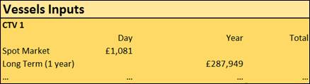
In order to perform the analysis the cost of each type of vessel considering various markets should be introduced. For example, the cost of jack-up under different financial options is displayed in Figure 12 below:
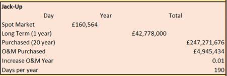
Figure 12: Jack-up Vessel Inputs
It is important to know that small CTV (less than 12 meters length) are not allowed to travel further than 60 nautical miles. A bigger CTV should be employed when the distance from shore is more than 60 nm. Therefore, these CTV will be more expensive, and this fact is also considered in our analysis:
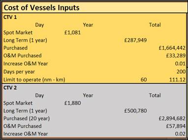
Figure 13: CTV Vessel Inputs
Cost of vessels. Preventive maintenance
The cost of vessels for doing preventive maintenance tasks is calculated for each solution (21 cases). Since there are particular excel sheets for no offshore accommodation, mothership and jack-up, this cost is displayed in the corresponding excel sheet. Moreover, the cost is calculated each year for every market:
- Spot market: The cost of hiring a vessel is multiplied for the number of the days required.
- One year charter: The cost consider is only one value per year, therefore, this parameter is constant when changing the days required.
- Purchased: The capital cost is included in the first year, afterwards only the operational cost is considered.
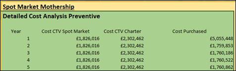
Figure 14: Cost vessels per year, preventive maintenance
Cost of vessels. Corrective maintenance.
As previously mentioned, corrective maintenance has been divided into five main categories. Small replacements cover three categories (A, B and C), and large replacements cover two categories (D, E). The actual downtimes (not including waiting time and logistic time) have been calculated previously, thus, the number of days required for both small and large replacements are already defined.
- Small replacements: It has been considered that CTV are employed during these operations. CTV should be hired from spot market based on the days required for performing small replacements. In case of charter or purchase, CTV which is available could be used for performing small replacements (in addition to preventive tasks). Then CTV will be hired from spot market just if the number of CTV available is not enough to carry out small replacements.
CTV Spot market:

CTV Charter or purchase:


- Large replacements: It has been considered that Jack-Up are employed during these operations. In case of no offshore accommodation, mothership or jackup-spot market, jack-ups should be hired from spot marker regarding the days required for performing large replacements. In case of jack-up charter or purchase, jack-ups which are available could be used for performing large replacements (in addition to preventive tasks), then more jack-ups will be hired from spot market just if the number of them available is not enough to carry out large replacements. These values are calculated in a similar way as for small replacements:
No offshore accommodation, mothership or jack-up spot market:

Charter or purchase:


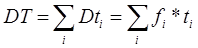
Finally, both small and large replacement vessel costs are summed up every year (since failure rates will change over time) in order to obtain the corrective vessel cost for each case the following equation is used:

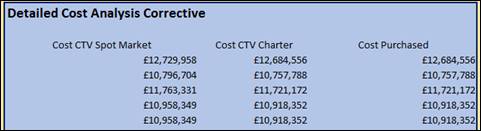
Figure 15: Cost of Vessels per year, Corrective Maintenance
Total Cost
The total cost includes the following:
- Cost of personnel
- Downtime cost
- Cost of vessels for preventive maintenance
- Cost of vessels for corrective maintenance
Those costs have been explained and calculated in the previous sections. The final cost considered for each case per year was determined by the following equation

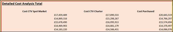
Figure 16: Total Cost of Vessels per year
Finally, an indicative graph has been incorporated within no offshore accommodation, mothership and jackup, representing the different cases when considering all the market possibilities. For example, in case of jack-up solution we get the following graph:

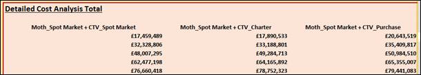
Figure 17: Total Cumulative Cost of Vessel per year
Finally, an indicative graph has been incorporated within no offshore accommodation, mothership and jackup, representing the different cases when considering all the market possibilities. For example, in case of jack-up solution we get the following graph:
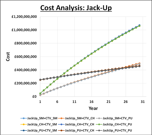
Figure 18: Cost Analysis of Jack Up Vessel
Sheet: Inputs
Since many inputs are required for the calculations, it has been considered to include all the inputs in a single excel sheet. Therefore, the user can modify every input from this sheet and all the values will be updated in the related location within the excel tool.
The inputs have been arranged into four main categories:
- Preventive Maintenance Inputs:
- Corrective Maintenance Inputs:
Moreover, within this sheet, the button panel was also added. This button allows you to move easily around between sheets as well as running the analysis by clicking “Calculate” button.
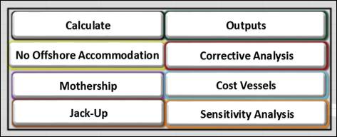
Figure 19: View of Interactive Tool Calculation Panel
Sheet: Outputs
As mentioned before 21 different solutions were considered. Thus, it would be difficult for the user to compare and choose the best solution for every case. In order to solve this problem, the minimum and maximum cost solutions are calculated and displayed using a Visual Basic code. In addition, another two potential solutions can be selected by the user in order to make fast comparisons.
The minimum and maxim cost solution are obtained when clicking the button “Calculate” inside the button panel. Every time the button Calculate is clicked, all the outputs will be updated automatically. The other two selected solutions [Select Solution 1, Select Solution 2] can be chosen using combo boxes:
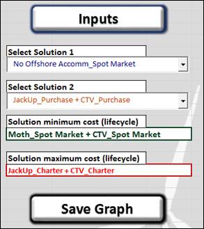
Figure 20: Outputs View 1
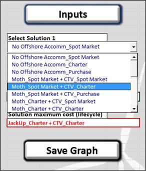
Figure 21: Outputs View 2
All the proposed solutions (maximum, minimum and two selected options) are displayed in the Cost Analysis Graph, representing the cumulative costs over certain amount of years. Also, there is a button for saving the graph as a picture, which allows fast and easy comparisons.
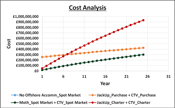
Figure 22: Cost Analysis Graph
Furthermore, specific figures from all the proposed solutions are also presented in order to provide a more detailed analysis.
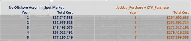
Figure 23: A Sample of Detailed Cost Analysis For Proposed Solutions
The Tool - Tutorial
Click on the following picture for a tutorial of the tool.
Remember to enable "CC" for the instructions.
Enjoy!