Case Studies
The following case studies will demonstrate the use of both the BoP cost and the Carbon cost tools. The first study will demonstrate that plant and turbine size affect the BoP cost and evaluate that the tool captures this. The second case study will evaluate the effect that changing location has on the BoP cost and again how the tool calculates this. The third Case study will investigate the environmental performance in terms of carbon cost in terms of balance of plant.
Cost Case Study 1
Cost Case Study 2
Carbon Case Study
Cost Case Study 1
Objective
The case study has been done to demonstrate the use of the BoP tool, examining how different wind farm sizes affect the cost of BoP and further evaluating the result of the tool.
Description
It is a conceptual case study which compares a 50 MW wind plant for three different turbine sizes (750KW, 2.5MW and 5MW), in the same location. The plants assumed to be located on a hill near Inverness (grid reference at centre NH312 441) as shown in figure 1, where according to the Department of Energy & Climate Change website the average wind speed is 10m/s.
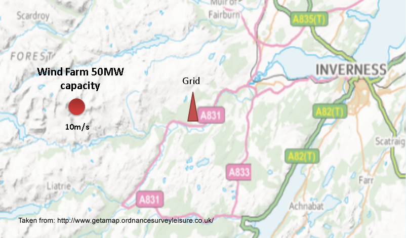
Figure1
We have developed conceptual wind farm layouts for three turbine sizes (figure 2). The 50-MW wind plant requires 66 of 750 kW, 20 of 2.5 MW and 10 of 5 MW-size turbines. turbines are arranged in a rectilinear array
The dimensions for wind farm turbines are presented in the table 1
Plant Size |
Rotor Diameter |
Minimum Distance Between Turbines |
Minimum Distance Between Rows |
MW |
m |
m |
m |
0.75 |
50 |
115 |
600 |
2.5 |
85 |
196 |
1,020 |
5 |
120 |
276 |
1,440 |
which have been designed to achieve the lowest possible cost of energy based on research that has been carried out by the National Renewable Energy Laboratory (NREL U.S. Department of Energy Laboratory).
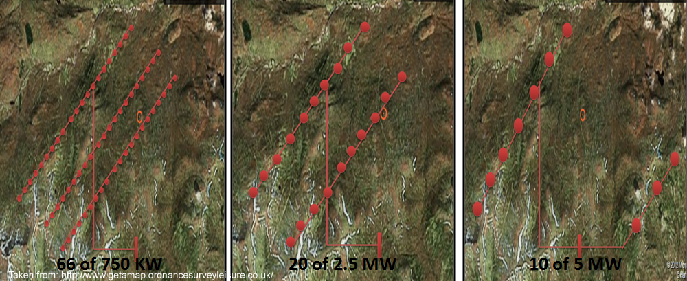
Figure 2
Results
By using the tool, the balance of plant cost has been obtained for each farm, where it has been observed that the cost decreases as the turbine size increases. For example, for the 750 kW the cost was the highest at £20.35 million while for the 5 MW size the cost of the plant decreased to £10 million (figure 3).
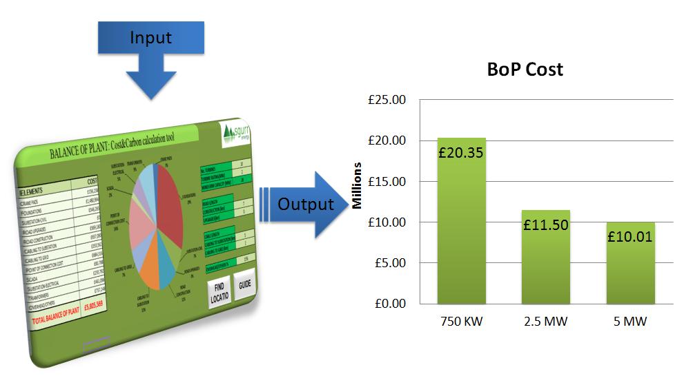
Figure 3
To calculate the annual power produced from the plants the capacity factor (Cf) has been obtained from the velocity ratio (Vr) curve, where at Vr equal to 2, Cf is equal to 0.32. Since the capacity of the plants are the same at 50 MW, the annual power production is 140 GWh/year and this will give around £6.5 million annually return (taking into consideration the price of energy displaced including feed in tariffs 4.7£/kWh).
To calculate the simple pay back, the initial cost of each farm has to be calculated. Based on current commercial turbine costs it has been found that each MW is equal to around £2 million. Therefore, the simple pay back is presented in table 2 below.
0.75MW |
2.5MW |
5MW |
|
Annual Energy Production (kWh/y) |
140,160,000 |
140,160,000 |
140,160,000 |
Annual Return (£/y) |
6,587,520 |
6,587,520 |
6,587,520 |
Turbines Cost (£ million/plant ) |
100 |
100 |
100 |
BoP Cost (£ million) |
20.35 |
11.5 |
10.01 |
Simple Payback (years) |
18 |
17 |
16.5 |
Table 2
Analysis & Discussion
Based on the tool results it has been noticed that the largest component of BoP cost is the foundations where it contributes about 32% to the total cost of the plant, the second largest component is the transformers by 13%. The contribution of cabling and road works were also high reaching 18% and 15% respectively (figure 4). It has further been observed that these items change dramatically when comparing the 750 kW plant with the 5MW. For example, the foundation cost reduced from around £8 million for the 750 kW plant to around £2 million, the transformers cost also showed a reduction from around £3.5 million to £1 million, and it seems that reducing the turbine numbers reduces the cabling and road works that contribute to reduce the total cost of the plant.
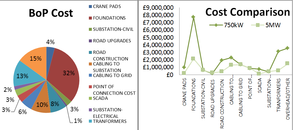
Figure 4
According to the data calculation it has been observed also that the cost of each farm can vary due to commercial aspects. The variation between different plants is also linked to the number of turbines selected, as the number of turbines increase in the calculation the percentage of uncertainty also increased. For example for the 750kW plant there was a big variation by around £15 million and only £5 million for the smallest farm (figure 4).
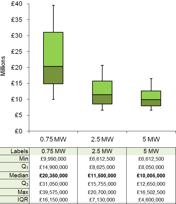
Figure 5
BoP Case Study 2
Description
It is a conceptual case study which compares two 50 MW wind plants of the same size but for different locations. The first location (old location) is the same the same for case study 1 (at average m/s wind speed and 5 km away from the grid), and the second (new location) is assumed to be closer to the grid ( 1km away from grid) but less windy with an average of 6 m/s. We have used the same turbines arrangement for the 2.5MW layout for the two locations.
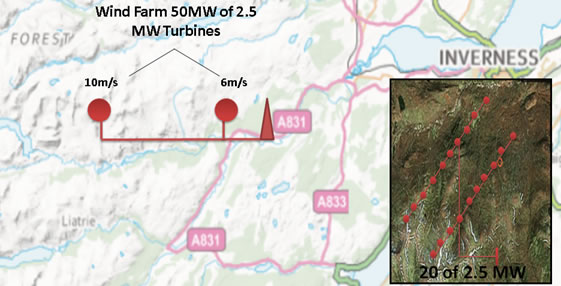
Figure 6 Location of the new plant.
Results
Again, by using tool the balance of plant cost has been obtained for each farm, where it has been observed that the cost decreases as the distance to the grid decrease. For example, for the old location the results are £ 11.5 million and £ 10.6 million for the second (see figure 7).
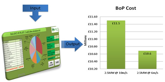
Figure 7 BoP cost calculations
Since we are comparing farms at different locations it is important also to look at the annual energy production of each plant. The calculations showed that the old location can deliver around 140 MWh as an annual energy production while the new location can deliver only around 122 MWh (see figure 8). This increased the payback period from 17 to around 19 years for the old and the new location respectively (based on 4.7£/kWh feed in tariffs rate).
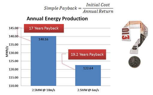
Figure 8 Annual energy production and simple payback.
Analysis & Discussion
Based on the obtained results it has been noticed, despite that the new location is cheaper in regards to BoP cost but the old location is still preferable because it has less payback years (17 years). Reducing the distance between the farm and the grid has reduced the cost associated with roads and cabling works and due to that reduced the total balance of plant cost. Changing the plant location has changed the subjected wind speed and as a result it has affected both the balance of plant cost and the annual energy production.
Carbon Case Study
Objective
The aim of the case study is to use the developed carbon cost estimating tool to evaluate the quantity of carbon emissions resulting from the construction of the BoP components. This value will then be assessed for its environmental performance represented by the carbon Payback and intensity indicators.
Description
A hypothetical wind farm was devised with probable quantities and types of construction materials encompassing the following parameters:
100MW wind farm consisting of 50 x 2MW turbines
capacity factor of 30%
Lifespan of 20 years
20km from grid connection
10km from Quarry (For aggregates, sand etc.)
20km from Metal works (For cabling, steel, etc.)
Foundations are 16m by 16m by 3m – Concrete with 5% average recycled steel
Crane pads are 20m by 40m – Aggregates and High Density Poly Ethylene (HDPE)
Onsite Roads 25km by 5m – Aggregates and HDPE
Cable Trenches 45km by 1m – filled with Sand and topped with excavated soils
Cables to Substation 25km by 50mm2 – Copper (general) and HDPE
Cables to Grid 20km by 250mm2 – Copper (general) and HDPE
Substation building 24 tonnes concrete and 0.01 tonnes steel
Transformer (none on site as transmitting at 11kV at grid connection)
Results of Case Study
It was found from these parameters that the total embodied and transported carbon for the BoP was 18,310 tonnes CO2e. By far the biggest contributor is the foundations, providing just over 55% of the total, followed by the onsite roads 15%, and then cabling to grid 14%.
The environmental indices were as follows; Carbon Payback 0.162 years and Carbon Footprint 3.48g CO2e/kWh.