
 Home
Home 
| HAMCT |
|
| VAMCT |
Hydrodynamics
Consider a 2D foil at some arbitrary angle and at zero angle to the freestream will experience a pressure distribution somewhat similar to the following diagram:
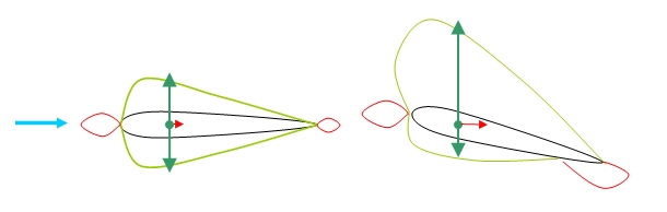
Pressure Distribution
The green lines indicate a negative relative pressure (suction)
and red lines positive, and the arrows indicate the resultant
forces associated with the pressure distribution. It should
be noted that as the angle of incidence increases, the bottom
surface may in fact experience a positive relative pressure.
The green arrows indicate the lift associated with each side
of the foil, and the red arrow indicates the drag associated
with the pressures. It should be noted that as pressure forces
act normal to surfaces that these arrows are the cumulative
forces of the pressure distribution integrated over the foil.
That this foil shown is symmetric is to indicate that the pressure
forces themselves are symmetric when the flow conditions are
symmetric, and the foil only generates “lift” in
one direction when it is cocked in that direction to the flow.
From US Navy Postgraduate School Dept. of Aeronautics
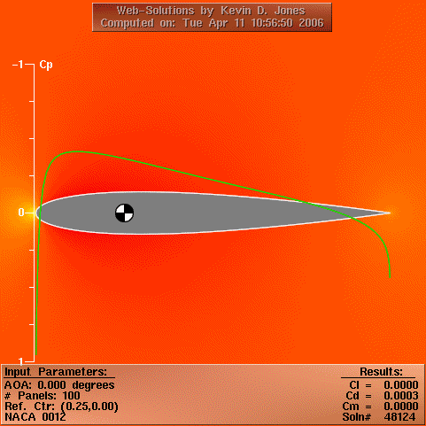
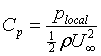
The local pressure may be non-dimensionalised by the free stream
dynamic head to yield the pressure coefficient CP, which varies
over the aerofoil.
The integrated sum of the pressure ever the foil yields lift and pressure drag (which is a constituent of overall drag). The lift is the useful output of the foil and drag merely wastes energy. Lift and drag may themselves be non-dimensionalised according to:
![]()
Where c is the chord length for the foil (distance
from tip to root).
These foil parameters are what define the characteristics of
an foil, and it should be noted that it is conventional to:
-
denote 2D section parameters in lowercase eg Cl not CL (reserved for full 3D foils)
-
denote Cp as negative upwards on pressure distribution diagrams (makes sense as negative Cp is on the lifting side of a foil)
- express section characteristics against foil angle of attack
As angle of attack increases, up until a point, the resultant
lift on the foil increases (almost linearly at ![]() per
radian) until the foil stalls, generally around 15 or so degrees.
Here there is a massive increase in drag and a decrease in lift.
per
radian) until the foil stalls, generally around 15 or so degrees.
Here there is a massive increase in drag and a decrease in lift.
It is these parameters that characterise the hydrodynamics of our generic devices. Since the devices are likely to experience local angles of attack much greater than 15 degrees, full range data has been acquired:
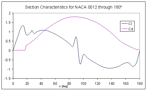
Results from (2)
It was decided for simplicity to use symmetrical NACA 00xx foils, and as such only section data between 0-180 degrees is required.
Cavitation
An instance where hydrodynamics and aerodynamics diverge is in the case of cavitation. This phenomenon is when bubbles of relative vacuum are formed when the local pressure of the fluid drops below the vaporisation pressure and in effect the fluid boils. In this circumstance the bubbles are convected to a region of relatively higher pressure where they spontaneously collapse at sonic velocity, which is sufficiently intense to cause structural damage such as surface pitting and integrity breakdown. The generation of lift by relative suction on the hydrodynamic top of a foil can result in localised pressure sufficiently low for this to occur.
The prediction of cavitation is a prime concern when choosing
foil sections, and can dictate the maximum rate of motion a turbine
blade may experience. In modeling the generic devices cavitation
was considered to occur if the local pressure coefficient dropped
below the fluid vaporisation pressure coefficient. Formally cavitation
occurs if:
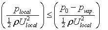 or
or ![]() where
where![]()
![]()
As such tendency to cavitate depends on local relative fluid
velocity, local dynamic pressure and local depth h. Therefore,
in the models requiring an upper limit to angular velocity, it
was considered that the device would operate at a minimum depth
of 5 metres, and that standard ISA conditions (101325 Pa atmospheric
pressure) and “normal” seawater characteristics (pvap=
0.6 kPa; ![]() =1027kgm3).
=1027kgm3).
The aerofoil minimum Cp was found from a panel method simulation (results animated above) for a range of angles of attack, and as such cavitation could be considered to limit the angular rate of devices when Cp was sufficiently low.
Betz Limit Review
A turbine placed in a fluid flow cannot be expected to convert all the kinetic energy meeting its blades into electrical energy, otherwise the turbine would essentially constitute an impermeable solid, damming the portion of water bounded by the swept area. The energy density of water is also much greater than that of air, but it is a much slower moving medium to harness for power generation. Consequently, tidal turbines exhibit what is referred to as high solidity, to capture as much energy as possible. That is, the chord length of the blades will be larger, and the blades shorter than those of a wind turbine. Generally, 3 bladed configurations of axial flow turbines are favoured, though two bladed versions are cheaper and easier to transport as they can be laid flat. If more than 3 blades are used it is thought that at higher rotational velocities tip wake interactions may occur, as each successive blade enters a turbulent region caused by the preceding blade’s movement.
So if the optimal blade configuration is assumed, what does constrain
the maximum extractable portion of the kinetic energy? Often,
the Lanchester-Betz limit is assumed
to describe the maximum attainable efficiency for both wind and
tidal turbines, and gives a power coefficient of 16/27, or 0.593,
though it has come to light in testing that this is not always
the case. Betz's theory describes how flow spreads out and slows
as it encounters the turbine, and pressure differences across
the bounded domain in conjunction with Benoulli’s theorem
gives rise to the axial induction factor, and subsequently permits
the calculation of thrust on the rotor blades. The axial induction
factor is a factor relating the flow velocity through the turbine
to the up and downstream velocities, and gives a maximum CP
when (it) ![]() =1/3.
Bernoulli’s theorem is applicable by assuming frictionless,
incompressible, lamellar flow in a 1D analysis, and that fluid
passing through the rotors is converted completely into a useful
form of work (4). In reality, power coefficients
in the region of 0.2-0.6 are likely for tidal turbines, and the
Betz limit describes the absolute theoretical limit of only wind
turbine efficiency.
=1/3.
Bernoulli’s theorem is applicable by assuming frictionless,
incompressible, lamellar flow in a 1D analysis, and that fluid
passing through the rotors is converted completely into a useful
form of work (4). In reality, power coefficients
in the region of 0.2-0.6 are likely for tidal turbines, and the
Betz limit describes the absolute theoretical limit of only wind
turbine efficiency.
Gorlov and the GGS model
There is another way though, the GGS model, named after its creators, Gorlov, Gorban and Silantyev, which describes the limitations of turbine efficiency in a very different way. The GGS model attempts to demonstrate how the Betz limit overestimates propeller type turbine performance in water, as it cannot compensate for the effects of flow separation. In this method a curvilinear pressure distribution can be applied to the rotor area, and the resultant thrust calculated (5). The mathematics is quite complex and uses divergence theory coupled with modified Kirchhoff flow, while assuming a degree of flow separation at the rotor’s perimeter, and suggest that the maximum attainable efficiency for an axial tidal turbine is little over 30%. However, the DTI state that their 300kW turbine used in the seaflow project recorded varying Cp’s, the highest of which was 0.6 (7), surpassing even the Betz limit - perhaps an anomaly, but it has also been suggested that these rules cannot be readily applied to marine situations. It has been stated that axial turbines might nominally display Cps from 0.2-0.4, cross flow turbines from 0.25 to the rather impressive Kobold turbine’s claimed 0.42, and a tried and tested 0.35 for the Gorlov helical turbine (5). It therefore becomes quite difficult to choose an efficiency to use for modelling purposes due to the diverse figures in literature, and how exactly this relates to the flow passing through the turbine at any given time. To allow for this, the models developed for this site allow the user to input their own parameters in a number of areas as less contradictory information arises. For the purposes of modelling, it was decided to use the generic models to ascertain efficiency values due to the ostensible uncertainty in this area, as it gives realistic efficiency figures, which will ensure resource overestimation will be minimal. For flow through the rotors at different efficiencies however, it was decided that GGS values for effective solidity would be used, as this constitutes very useful information for calculating SIF effects. For progressive work or improvements to the SIF model, it would be pertinent to investigate further effective solidity, and use more accurate data for parametric timestep SIF calculation as it becomes available.
Vortex Wake Analysis
Since a sphere of influence type analysis dictates that turbines must be spaced some significant distance from one another in the lateral sense, it is interesting to try and quantify the absolute minimum distance that would be appropriate, if backwater and blockage effects could be assumed fairly negligible. This may be achieved by consideration of the vortex wake structure for the turbine.
A foil shaped blade generates lift by a pressure difference over is streamwise upper and lower surfaces. This pressure difference gives rise to “leakage” around the front and edge of the foil, which in turn develops into a bound circulation. One way to visualise this is to consider the velocities at any point on the surface be made up of the mean velocity of all points plus (or minus) some circulatory component: on the upper surface where the flow is faster due to foil shape (for an asymmetrical foil) or the presence of a stagnation point on the bottom surface (for a symmetrical foil) the circulation component increases local velocities from the mean in a rearward direction. Conversely, on the lower surface, the flow is retarded from the mean by the circulatory component. Considered in isolation, this circulatory component gives rise to a bound vortex on the foil.
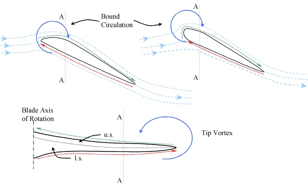
At the blade tip, a similar leakage induces a vortex about the
blade tip. This rotation is convected downstream by the flow,
and generates the famous trailing vortices seen behind aircraft
wings. It’s presence causes a similar circulation around
the upper and lower surfaces of the blade in a spanwise direction,
and as such the bound circulations are linked. According to Helmholz’s
theory on vorticity, a vortex can neither begin nor end in a fluid,
and as such is conservative; it may form a closed loop; is carried
by the flow.
Bound circulation and lift (l) on a 2D foil may be linked as follows:
![]()
with![]() being the strength (magnitude) of the bound vortex whose axis
is perpendicular to the flow and the chord.
being the strength (magnitude) of the bound vortex whose axis
is perpendicular to the flow and the chord.
Due to Helmholz and the conservation of angular momentum, when
the foil lift is integrated to give the blade performance one
may say that the strength of the trailing vortex (“made
up” of the discrete bound circulations) may also be related
to blade lift. Couple this with the initial starting vortex of
the blade (which itself allows the conservation law to be obeyed)
and the vortex strength of the wake may be determined.
Biot-Savart Integration
Biot-Savart’s Law was originally derived to calculate the
magnetic field strength at a point about a charge carrier or other
potential (eg a wire), but has been adopted as a solution to the
case of a filament vortex in fluid dynamics.
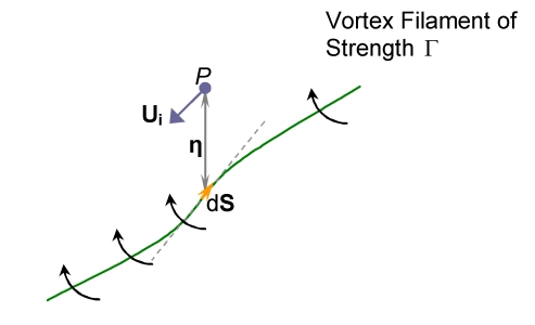
The law relates the velocity induced by a filament of vorticity
at an eccentric point to the vortex strength and the position
of the point. For the infinitesimal element of a filament of vorticity
of strength ![]() the
induced velocity on point P at position
the
induced velocity on point P at position![]() from element dS is given by
from element dS is given by
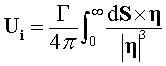
For all elements between the start of the filament and infinity.
Now, considering the assumptions made during the derivation of
actuator disk theory (infinite number of infinitesimal blades)
it may be postulated that the tip vortices at the root form a
central core vortex along the axis of the rotor disk, and that
the tip vortices are sufficiently close together that they coalesce
into a cylindrical vortex sheet. Further, the helical nature of
the trailing vortices may be modelled as a number of ring vortices
and axial vortices, themselves coalesced into a sheet, and as
the physical problem is the same, replacing the original wake
sheet. It is the induction effects of the ring vortices which
are of chief concern, as it is these which alter the axial velocity
of the flow in the wake, which, by conservation of mass, alters
the wake diameter and hence device spacing.
Assuming an axisymmetric wake (e.g., no rotor yaw) the analysis proceeds as follows, considering this schematic of the problem geometry:
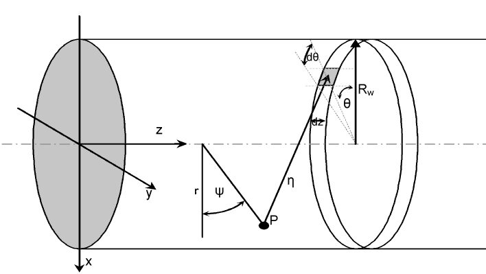
Since the effect of the rotor is to retard the flow, conservation
of mass dictates that the radius of the wake, Rw, will
increase so that the mass flow rate is constant. Thus if the axial
velocity can be calculated at every point at a certain axial station
z then the mass flux through the area may be calculated. We use
the integral relation:
| Eqn. 1 |
where ![]() is
the axial velocity calculated at each radial position which is
reduced from the freestream by Ui,z. Recasting the
Biot-Savart Law into differential form:
is
the axial velocity calculated at each radial position which is
reduced from the freestream by Ui,z. Recasting the
Biot-Savart Law into differential form:
 |
Eqn. 2 |
In a basic calculation, as proposed by Coleman (13),
the wake is purely cylindrical of consant radius, and the vortical
strength ![]() is
constant along the wake. Furthermore, in Coleman’s analysis
for the strength to be constant the far wake strength must be
equal to twice the far wake induced velocity:
is
constant along the wake. Furthermore, in Coleman’s analysis
for the strength to be constant the far wake strength must be
equal to twice the far wake induced velocity:
![]()
Circulation per unit length of the vortical filament given by:
![]()
where the term in parenthesis is the streamwise convection velocity in the far wake and satisfies the limit above. Uz,P is the axial velocity at point P and is calculated at each step.
The integration of the Biot-Savart law (eqn 2) yields all values required, but is an iterative process. The iteration is begun with the Coleman model which stipulates constant vorticity and wake radius, from which the calculation proceeds as follows
- The results from actuator disk theory yield

- Eqn 1 is used to calculate mass flow at a number of z-wise stations
- The wake radius at each station is linearily stretched so as to accommodate conservation of mass
- New vortex strength distribution is then calculated around the ring vortex found at each z-wise station.
- Eqn 2 is integrated at each z station in and r using the new
approximate wake properties yielding new
- Repeat from 2
The iteration proceeds until a converged solution is reached, however it was found that computational time is excessive at relatively fine wake gridding intervals, so the process was only allowed to run for 15 iterations in each case. Also, since the Biot-Savart relation must be integrated up to infinity, z ordinates were chosen on a logarithmic scale up to a point where the wake was considered fully developed, from where the integration was performed analytically. The algorithm was implimented in a Matlab script and may be downloaded as part of the generic HAMCT package from the tools page.
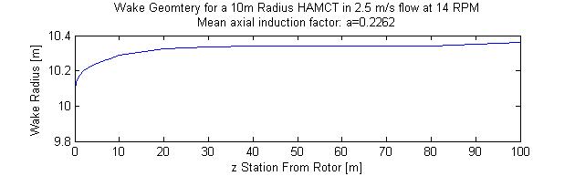
As can be seen from the results of the model, at even a rip-roaring
tidal flow velocity of 2.5ms-1 the wake is virtually
fully formed (99%) within half a diameter of the rotor, and it
can be seen that the wake is only .3 or .4 of a meter on top of
the radius of the blades themselfves. Thus, it appears that at
a push wake induction interaction (as each velocity at the rotor
depends on the entire wake) is not going to occur unless the turbines
are exceptionally close together.
References
| 1 | MUNSEN, B., et al., Fundamentals of Fluid Mechanics. 3 ed. 1998, New York: John Wiliey & Sons. pp. 877. ISBN |
| 2 | KLIMAS, P. and SHELDAHL, R., SAND80-2114: Aerodynamic Characteristics of Seven Symmetrical Airfoil Sections through 180-Degree Angle of Attack for Use in Aerodynamic Analysis of Vertical Axis Wind Turbines, 1981 Sandia National Laboratories, Albuquerque |
| 3 | MOLLAND, A.F., et al., Measurements and Predictions of Forces, Pressures and Cavitation on 2-D Sections Suitable for Marine Current Turbines. Proceedings of the Institution of Mechanical Engineers Part M: Journal of Engineering for the Maritime Environment, 2004. 218(2): p. 127-138. |
| 4 | DAVIES, P., Warwick Univeristy ES427: The Natural Environment and Engineering: Global Warming and Renewable Energy Lecture 4: Wind Energy. [PDF] 2002 [cited 03 May 2006]; Available from http://www2.warwick.ac.uk/fac/sci/eng/staff/pad/teaching/lecture4.pdf |
| 5 | GORBAN, A.N., et al., Limits of the Turbine Efficiency for Free Fluid Flow. Transactions of the ASME Journal of Energy Resources Technology, 2001. 123(4): p. 311-17. |
| 6 | THAKE, J., DTI Renewables: Development, Installation and Testing of a Large Scale Tidal Current Turbine. [PDF] 2005 [cited 02 May 2006]; Available from http://www.dti.gov.uk/renewables/publications/pdfs/t060021rep.pdf |
| 7 | MAGNUSSON, M. and SMEDMAN, A.S., Air Flow Behind Wind Turbines. Journal of Wind Engineering and Industrial Aerodynamics, 1999. 80: p. 169-189. |
| 8 | THOMSEN, K. and SORENSEN, P., Fatigue Loads for Wind Turbines Operating in Wakes. Journal of Wind Engineering and Industrial Aerodynamics, 1999. 80(1-2): p. 121-136. |
| 9 | VERMEER, L.J., et al., Wind Turbine Wake Aerodynamics. Progress in Aerospace Sciences, 2003. 39(6-7): p. 467-510. |
| 10 | WANG, T. and COTON, F.N., Prediction of the Unsteady Aerodynamic Characteristics of Horizontal Axis Wind Turbines Including Three-Dimensional Effects. Proceedings of the Institution of Mechanical Engineers, Part A (Journal of Power and Energy), 2000. 214(A5): p. 385-400. |
| 11 | WHALE, J., et al., An Experimental and Numerical Study of the Vortex Structure in the Wake of a Wind Turbine. Journal of Wind Engineering and Industrial Aerodynamics, 2000. 84(1): p. 1-21. |
| 12 | CHANEY, K. and EGGERS, A.J., Expanding Wake Induction Effects on Thrust Distribution on a Rotor Disc Wind Energy, 2001(5): p. 213-226. |
| 13 | COLEMAN, R. et al., NACA ARR No. L5E10: Evaluation of the induced-velocity field of an idealized helicopter rotor. 1945 NASA Langley |
| HAMCT |
|
| VAMCT |
Go back to Contents