
The only exception to this was when sufficient data was available, instead of annual velocity exceedence curves, seasonal curves were constructed. Three equivalent power duration curves were then constructed for each season.
This meant a total of 12 curves had to be constructed for each set of wind data but allowed a more detailed examination of turbine performance and comparisond between the three machines to be made.
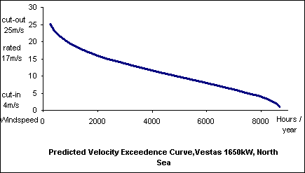
Velocity Exceedence Curve
For the North Sea, 'c' and 'k' parameters were available. In this case the Weibull distibution was used and the probability of windspeed exceeding any specific value could be calculated. From these probabilities a velocity exceedence curve was constructed - by multiplying the probability of exceeding a particular value of windspeed by 8650 (the number of hours in a year).
Where 'c' and 'k' values were not available, as with the rest of the world, a Rayleigh distribution was assumed. This enabled the probability of windspeed exceeding any specific value to be calculated and so a velocity exceedence curve could be constructed.
It was sufficient for calculation purposes, in both the above cases, that the velocity exceedence curve be evaluated only for whole number windspeed values (i.e at 3m/s, 4 m/s, 5m/s,......) since in most cases the wind data was coarse and because the available wind turbine performance data was given at this resolution.
This process was repeated, a velocity exceedence curve was constructed for each area of interest - just about every offshore oil field in the world.
Performance data for the three largest commercially available wind turbines was available. These were
From the velocity exceedence curve it was known, statistically, for how many hours it was likely to exceed a certain value of windspeed in the location where the data was measured . Included in the wind turbine data was the response curve, giving expected power generation over the operating range of windspeed. It was then simple to correlate m/s to kW (number of hours per year exceeding a value of windspeed to the generated power at that windspeed), the number of hours that the machine was expected to generate this power being the same as the number of hours that windspeed was expected to exceed that value of m/s.
Evaluating this over the operating range of the wind turbine enabled the equivalent power duration curve to be constructed. This was evaluated at the same windspeeds as the velocity exceedence curve. An estimation of the expected yearly output of the turbine could then be calculated by integrating (numerically) the area under the equivalent power duration curve.
The same method was used for calculating equivalent power, independant of the method of calculating velocity exceedence.
For each of the calculated wind profiles (velocity exceedence curves), the equivalent power duration curve was constructed.
In fact three equivalent power duration curves were constructed and integrated for every wind profile - one for each wind turbine considered.
Wind Data
One of the major challenges of this project was not only evaluating a large number of velocity exceedence curves but actually sourcing wind data to work with in the first place.
This means that where we evaluated wind resource using the global dataset, the results are suitable for an initial assessment of the wind resource of offshore oil fields world wide (and therefore the feasibility of wind energy conversion in that region) it is a relative more than definitive assessment and care should be taken.
North Sea Dataset
Wind data for offshore UK was available from various sources but for consistency we chose one source, which gave 'c' and 'k' parameters.
European Dataset
Wind data for Europe was readily available online from Riso in the form of 'The European Offshore Wind Atlas'.
USA Dataset
Wind data was also available for North America in the form of "Wind Energy Resource Atlas Of the United
States".(Produced by Pacific Northwest National Laboratory) - which is a land atlas but does include some near shore data..
Global Dataset
Initially we could find no other consistent or good quality data for the other regions we were interested in, namely South America, Australia, Indonesia, Africa and Canada. We finally managed to source data for these continents in Pilots Volumes, which were available in the University library and contained consistent and good quality (it was official Met Office, if slightly dated) data.
The limitations of this source were that it gave only mean wind speed and not shape, 'k'. Also the data was only for coastal stations, there was no offshore data of good quality.
Dataset Comparison
We compared our three offshore data sets (Europe, North Sea, USA) with our global data set to examine how consistent they were. When we compared coastal data from pilots volumes with figures from offshore - we did this for the North Sea, the Mediterranean and California - we found a relative increase in windspeed of between 10% and 20% when moving offshore. This is consistent with the the increase normally expected.
 Wind Menu