Optimising Spin Ratio
This page describes how the power savings of each trip were calculated, with a focus on how the operation of the Flettner rotor would be optimised for maximum power generation (this would usually be completed by the control system of the Flettner rotor).
Finding the Optimal Spin Ratio
From the theory section it is known that spin ratio (SR) has a significant impact on coefficients of lift and drag, and thus controlling the speed of rotation is the primary method of optimising rotor operation.
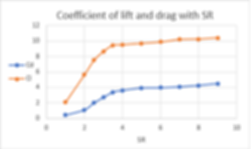
As previously explained in the CFD study section, a reliable relationship between coefficients of lift and drag have been obtained from (Da-Qing, et al., 2012). The plot has been digitalised and is shown below, with great care taken to precisely match the points on the graph
Obtained from ECMWF, the range of weather data varies between 1 and 24m/s and at a variety of angles. Given that the rotor has an operational range of up to 180rpm, there is a wide range of possible SR, and it is important to maintain the optimal SR that gives the most power saving. The above graph shows relationship between C_L, C_D, and SR, but the goal is not to minimise drag and maximise lift as it would be for a standard aerofoil, the output we would like to maximise is the thrust coefficient, C_T, as taken from the forward thrust equation presented in the background theory:
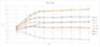
So we can see it also varies with angle of attack, α. This coefficient was plotted on a graph against spin ratio for different angles of attack ranging from 0-180°. The relationship mirrors itself from 180-360° as the rotation of the rotor would reverse its direction so there is no need to show angles above 180°, i.e. 150° would give the same result as 210°, 100° the same as 260° as they are the same difference in degrees from 180°.
The coefficient of thrust is seen to be closely affected by angle of attack and SR. For the majority of angles of attack C_T reaches a “plateau” around a SR of 3.5 so this is expected to be the optimal SR for maximising power savings.
Given the exponential relationship between power consumed by the rotor and rotational frequency, f (in rpm) from the graph in the power calculations page:
After the plateau in C_T at SR of ~3.5, a small increase in C_T (from an increase in SR) would be outweighed by the additional power consumed to increase the rotor’s rotational frequency to the higher SR.
Therefore there is an ideal SR, and although the majority is expected to be 3.5, it will change depending on the angle of attack. It can be seen on the graph of C_T against SR that an angle of 30° will not have an optimal SR of 3.5, and instead a SR of 2 would be preferred. To better represent this complicated relationship, the power savings formula was expanded and reduced to the variables as shown.
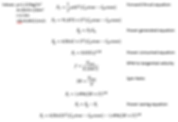
Notation is as follows: density (ρ), projected area (A), radius (r), apparent wind speed (U), boat speed (Ub), thrust force (FT), lift coefficient (C_L), drag coefficient (C_D), angle of attack (α), power generated (Pg), power consumed (Pc), power saved (Ps)
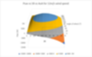
This newly calculated equation shows power saving as a function of five variables, C_L, C_D, U, SR and α. However, C_L and C_D both are defined by spin ratio, so this relationship can be considered to have three influencing parameters: SR, α, and U. The power saving for each wind speed can then be plotted on a 3D surface graph. Below is the graph for a wind speed of 12m/s.
Although true for any wind speed, the graph for a wind speed of 12m/s is presented as it clearly illustrates a peak SR of 3.5 for the majority of angles. It can be seen that angles below ~50° it seems that as angle of attack reduces, so does the optimal SR.
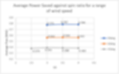
This was investigated further by comparing the average power saving of the rotor over a range of wind speeds (1-24m/s) for different SR and angle of attack, shown below.
The graph below shows that a SR of 3.5 gives the peak power saving for angles 60° and 90°, but not for an angle of 45°. This correlates with the earlier graph of CT vs SR from which it was obvious that 30° would not have an optimum SR of 3.5 and instead would be closer to 2. It has been proven here that this also applies to angles up to somewhere between 45-60°. Matching the optimal SR for angles in the range of 45-60° was assumed to give negligible impact on end results due to the minute differences in power savings (shown in grey on the above graph). For angles lower than 45° this was investigated further.
It is expected that the optimum spin ratio will vary for each angle in the range of 0-45° and is also dependant on the wind speed. Without more sophisticated software to handle these changing relationships, mapping and matching this peak SR would be a misuse of the limited time available in this project. A SR of 2 for angles less than 45° was tested, however, proved to have no impact on the end results. Therefore the difference in power savings between the optimal SR and a SR of 3.5 for angles less than 45° is no longer considered as it has been shown to be negligible.
To summarise, the relationship between coefficients of lift and drag and spin ratio were taken from (Da-Qing, et al., 2012). This relationship was incorporated with the range of wind speeds, and angles of attack that were present in the weather data obtained from ECMWF. This was studied in detail and presented in a variety of ways and the optimal spin ratio of 3.5 was confirmed for the data in this project. In cases where this spin ratio was not optimal, the difference in results was decidedly negligible.
High Wind Speed Cases
The wind data for the chosen dates gave apparent wind speeds ranging from 1-24m/s. Therefore the chosen SR of 3.5 could only be achieved up to wind speeds of ~13m/s, due to the maximum rotational frequency of 180rpm (giving a tangential velocity of 47.2m/s) as specified by (Norsepower, 2018). At wind speeds higher than this the rotor maintained its maximum frequency of 180rpm, which resulted in the SR for these cases dropping as the wind speed increased. To accurately match coefficients of lift and drag to SRs not specifically recorded from (Da-Qing, et al., 2012) the equations of trendlines were created for 0≤SR≤3.5 and are shown below.
Using a series of excel spreadsheets, the SR was set as 3.5, or as close to 3.5 as possible. Where 3.5 was achievable, the corresponding recorded C_L and C_D values were used. Where a lower SR had to be used because of the speed limited to 180rpm, the equations from the graph above were used to calculate the coefficients at that SR. Combining the apparent wind speeds and angles of attack (found using the methods described on the wind data page), and their corresponding SR and coefficients of lift and drag (as explained in this page), the power saving for each point of each journey of each month can be calculated using this equation:
The results of these calculations can be found on the results page.