CFD Study
This section gives extensive detail into the CFD process completed for this project. As explained in this page, the work was not able to be used for the project due to the chosen method not capturing specific flow phenomena. Results from a reliable and appropriate paper have been digitised by an online plot digitiser and the relationships between coefficients of lift and drag, and spin ratio are taken from this source and are presented at the beginning of the "Optimising Spin Ratio" page. Regardless of output, the following CFD process shows good practice for similar studies and would be valuable to other researchers of Flettner rotors using CFD.
Computational Fluid Dynamics (CFD)
CFD is specialised software that simulates fluid flow problems by using a combination of mathematics, numerical analysis and data structures to solve the famous Navier-Stokes equations. The software now plays a major role within the engineering and science community. However, the software is not 100% reliable, due to several factors such as the random motion of turbulence, parameter assumptions, inadequate mathematical model and computing power available. The main differences between experiments and CFD simulations is that experiments describe flow phenomena using measurements, whereas simulations numerically predict flow phenomena. The robustness of CFD software allows insight into fluid flow problems which are either too expensive or impossible to conduct using traditional methods. The software does not replace these methods but instead is used in conjunction with physical tests to enhance study results (Irvine, 2018). This study aimed to generate the relationship between coefficients of lift and drag and spin ratio for the chosen Flettner rotor for this project.
Main Study
The study presented is performed on the academic version of ANSYS FLUENT v19.2. A personal computer (PC) containing an Intel® Core ™ i5-4210M CPU @ 2.60GHz, with a usable installed RAM of 15.9 GB, 2 cores and 4 logical processors was used. Due to the computationally intensive requirements of 3D simulations with large element counts (> 2million) and the ANSYS academic element limit of 512000 it was decided a 2D study would be an acceptable approach. As the problem is simplified to a 2D model it is assumed that the PC has sufficient computing power and therefore not a limiting factor in study results (Irvine, 2018).
In order to determine power savings of the 30x5m Flettner rotor, coefficients of lift (Cl) and drag (Cd) against spin ratio (SR) must be identified to allow thrust to be calculated. As previously mentioned, SR, aspect ratio (AR) and Thom Discs are crucial variables affecting lift and drag. AR is constant at 6 and Thom discs are neglected as a 2D study is performed.
One journal article showing flow past a rotating 2D cylinder by (Gadkari, et al., 2017) was chosen to validate the present study’s results because the graphs of Cl and Cd demonstrate the popular trends seen in many 3D studies such as: (Marco, et al., 2016), (Pearson, 2014) and (Craft, et al., 2012). However, several important setup procedures such as boundary conditions and the turbulence model are not mentioned, therefore certain settings are validated from the three cited 3D studies. This made the following project as accurate and realistic as possible for a 2D study.
CFD Analysis Process
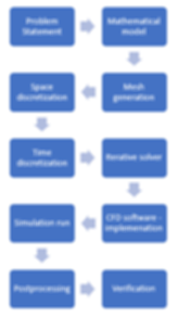
The above flowchart highlights the CFD analysis process. In laymen’s terms: a computer model of the problem is set-up, a mesh is generated, steady or time-dependant solver selected, boundary conditions and physics set-up (including turbulence model and pressure velocity coupling method) are specified, the simulation is run, and finally results are validated against benchmark data.
Computational Setup
The 2D computer model of the rotor and the fluid domain was built to a scale of 1:1 in ANSYS Designmodeler, replicating the dimensions used by (Marco, et al., 2016) for the fluid domain. The figure below illustrates the configuration of the computational domain.
To map out SR’s a freestream wind speed of 5 m/s was assigned to the inlet while the rotor’s RPM was altered accordingly to generate SR’s from 1-4. Using the equation U_tan=rω a 5m/s tangential velocity is equivalent to 19.1rpm. To evacuate air, a pressure outlet with a constant gauge pressure of 0 Pa is applied. To ensure zero-gradient conditions, the top and bottom of the computational domain are set to symmetry. This represents slip conditions, while the rotor is considered a rough wall (with non-slip conditions) and is set as a moving wall which rotates clockwise.
Mesh Generation
Generating the mesh is arguably the most important and difficult step in the CFD analysis process. Concentrating the mesh elements around and downwind of the rotor is key for accurate results. Generally, as the number of elements increase, the overall results improve, until an optimal level is achieved. Normally a compromise between number of elements and acceptable accuracy is performed. As a mesh becomes finer, the computational time required for simulations to converge increases (Irvine, 2018). The benchmark paper by (Gadkari, et al., 2017) fails to describe mesh refinements, therefore an independent mesh density study is performed. The figures below show the mesh set-up utilised for the present study against that of (Gadkari, et al., 2017), respectively.
Present Study Mesh
Mesh used by (Gadkari, et al., 2017)
Although differences are clearly seen when comparing the above meshes a similar approach was adopted and therefore deemed sufficient. Unstructured triangle elements make up the majority of the fluid domain in both cases with quadrilateral elements used, in the form of an inflation layer, to surround the rotor. Two body size functions were used to smoothly increase the mesh density towards the rotor applying a soft setting thus allowing a gradual change between borders A-B, and B-C. The ANSYS manual states that adjacent elements should not vary by more than 20%, and exceeding this can drastically lower mesh quality (Irvine, 2018). An inflation layer creates a smooth layer of elements running parallel across the surface of the rotor. The number of layers and growth rate vary depending on simulation, between 15-40 and 1.15-1.2, respectively. The First Layer Thickness (FLT) setting was utilised for the inflation layer to accurately set the first cell height adjacent to the rotor achieving the desired y^+ value.
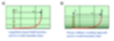
In order to achieve successful simulations, it is essential that calculations in the near-wall regions are as accurate as possible. y^+ is a non-dimensional distance describing how coarse or fine a mesh is, near the domain walls i.e. the rotor wall. Turbulence models have restrictions on the y^+ value: the most widely used turbulence schemes are k-ε and k-ω they typically work best at values 1 < y^+ < 5 or 30-50 < y^+ < 300 as stated by ANSYS (ANSYS, 2018) (ANSYS FLUENT, 2014). All simulations for the present study will use SST k-ω turbulence model. This model differs slightly to that of k-ω model, results tend to be more accurate for separated flow under adverse pressure gradient and it is one of the conventional models for aerofoil simulations throughout the CFD industry. The paper by (Marco, et al., 2016) utilises this scheme. There are two approaches that can be used when creating a mesh near walls: 1) Log based Wall Function (30-50 < y^+ < 300) or 2) Resolve the Viscous Sublayer (y^+≈1). Both approaches are tested via the independent mesh density study, and the Figure below shows a visual comparison between the two approaches 1) and 2).
It should be noted that y^+ should not be between 5 and 30. Simply, if 5 < y^+ < 30 then ANSYS will attempt to solve what’s known as the Buffer zone or the Transition layer, rather than the viscous sublayer or the log-law zone as shown in the following figure (from here on referred to as the velocity profile). A wall function would be imprecise, and the first cell would not be small enough to accurately predict the velocity gradient across the boundary layer (ANSYS, 2018).
Physics Set up
After generating the mesh, physics can be applied to the problem. Double precision and parallel processing options were utilised. Selecting parallel with four processes allows the calculations to be shared between cores, which reduces simulation time. The pressure-velocity coupling is achieved using the coupled scheme. The SIMPLE algorithm could have been used, however by trial and error the coupled method provided faster solution convergence. The convective terms are discretized using second order upwind accuracy (Karabelas, et al., 2012). This is done to minimise numerical diffusion. These setting are computationally more demanding than first order upwind method, however a higher degree of accuracy can be achieved with second order. Only pressure has the standard setting employed, with the table below summarising the solution methods used for each simulations. Convergence criteria (CC) for the residuals were set to 5e-5, which is considered adequate, and monitors for coefficients of lift and drag were appropriately setup.
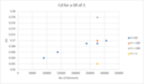
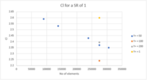
The results of the mesh density study are detailed below for a SR of ½ and 1. Initial only a y^+ of 50 was considered and therefore only recorded in the table below. However, y^+ = 1, 100, and 200 were also simulated at an element count of 275,000 allowing a comparison, this is seen in the graphs for a SR = 1. A high mesh quality is crucial to acquire realistic results. To examine the mesh, the inbuilt quality checker is utilised. The table below can be used to gauge the quality of a mesh. Skewness (Skn_max) and orthogonal (Oth_min) checks are commonly used for an unstructured mesh (Irvine, 2018).
It can be seen from the above graphs that Cl and Cd level off with increasing number of elements. Varying the y^+ value does show the sensitivity of the mesh around the rotor, however, no large offset is observed and therefore a y^+ of 50 at an element count of roughly 250,000 were employed for the remainder of this study.
Validating Results against Benchmark Data
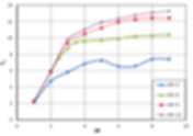
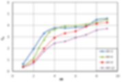
Below are the results of Cl and Cd against SR. A linear relationship can be seen between Cl and SR however, results similar to (Gadkari, et al., 2017) were expected. The vast majority of published articles show a similar trend were Cl levels off with increasing SR. The results for drag show worrying results too, the relationship of Cd is comparable with increasing SR however a large offset is observed.
Extensive research was conducted in an attempt to explain the discrepancies between present study results and benchmark data. It was found that some special circumstances occur for 2D studies at very high Reynolds Number (i.e. the turbulent flow which surrounds the Flettner rotor).
-
“when the vorticity on the cylinder’s surface accumulated large enough, it would pass through the closed flow line under the effect of centrifugal force and then exfoliated towards the wake. So, the lift coefficient would exceed 4π” (Yao, et al., 2016)
-
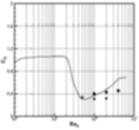
After Re > 2e5 a phenomenon called the ‘drag crisis’ takes place. Up to a Re of ~2e5 the boundary layer remains laminar but with increasing wind speed and thus Re even the viscous sublayer becomes fully turbulent (refer to the velocity profile figure for boundary layer zone reference). The point of separation therefore moves further from the rotor, producing a narrow wake and a large drop off in Cd (see the figure below).
However, it was explained by (Yao, et al., 2016) that even at very high Re experimental results and 3D CFD results would witness Cl levelling off with increasing SR and would avoid the drag crisis due to the influence of strong 3D effects caused by tip vortices. It can also be concluded that a 2D study would have been sufficient if Re was low enough. (Yao, et al., 2016) performed a 2D numerical study at similar Re’s to this study, with their results included in the graph of Cl against SR as black dots, notice the likewise trend.
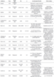
Since the 1900s the vast majority of papers address low Re rotating cylinder flows for industrial research of spinning machinery by numerical, experimental and theoretical methods (Yao, et al., 2016). See the table below for a summary of previous studies (Johnson, 2011).
A 5m diameter rotating Flettner rotor exposed to sea conditions will experiences far higher Re than any study mentioned in the table above. Although some papers do indicate that Flettner rotors will experience greater Re’s than the value selected for their research. For example, the report by (Johnson, 2011) utilises a Re of 140,000 believing it to be sufficiently high. The main reason papers opt for low Re conditions is for the validation of their results against experimental data, however, this may cause inaccuracies in results.
If we take the lowest operational wind speed of 1m/s and the highest 24 m/s recorded across the North Atlantic for this study, then Re is in the range of 3.4e5≤ Re ≤8.2e6. The table below characterises Re flow around a cylinder, it can be seen that most of the simulations for this project obtain a Re in the Supercritical/Transcritical Regime (Heseltine, 2003).
Although many papers have been published on Flettner rotors very little has been done to investigate the effects of Re > 1e6, this is mainly due to the lack of machinery experiencing very high Re so there was no need to investigate. However, today with the increase in size of engineering structures it is far more relevant. As the present study generated unrealistic results of Cl and Cd an alternative solution was adopted to allow the project to continue.
Fortunately, after widespread research a single paper was found with the help of Prof. Stephen Salter from Edinburgh University which met the requirements of the present study. “The Performance and Vortex Formation of Flettner Rotors At High Reynolds Numbers” by (Da-Qing, et al., 2012) was used. The paper utilises a 3D numerical study at full scale Re of 1.6e6 and at an AR of 6, therefore their results for Cl and Cd would represent our case accurately. It should be noted that with less of a time constraint a 3D study would have been attempted for the project. The results of Cl and Cd against SR by (Da-Qing, et al., 2012) are presented below and are used for the remainder of this project.
References
ANSYS FLUENT, 2014. Turbulence Modeling, Canonsburg: ANSYS Inc.
ANSYS, 2018. Student Community. [Online]
Available at:
[Accessed 12 April 2019].
Clayton, B. R., 1985. BWEA initiative on wind assisted ship propulsion (WASP). Journal of Wind Engineering and Industrial Aerodynamics, 19(1-3), pp. 251-276.
Craft, T. J., Iacovides, H., Johnson, N. & Launder , B. E., 2012. Back to the future: Flettner-Thom rotors for maritime propulsion?, Manchester: University of Manchester.
Da-Qing, L., Leer-Andresen, M. & Allenstrom, B., 2012. The Performance and vortex formation of Flettner Rotors at high Reynolds numbers. Gothenburg, 29th Symposium on Naval Hydrodynamics.
Gadkari, M. et al., 2017. To study Magnus Effect on Flettner Rotor. International Research Journal of Engineering and Technology, 4(2), pp. 1597- 1601.
Heseltine, J. L., 2003. Flow Around a Circular Cylinder with a Free End, Saskatchewan: University of Saskatchewan.
Irvine, R. A. M., 2018. A CFD STUDY ON THE EFFECTS TREES HAVE UPWIND OF A 5MW HAWT , Dundee: University of Dundee.
Johnson, N. D., 2011. High-Reynolds Number Flow Past a Rotating Cylinder With and Without Thom Discs , Manchester: University of Manchester.
Karabelas, S. J., Koumroglou, B. C., Argyropoulos, C. D. & Markatos, N. C., 2012. High Reynolds number turbulent flow past a rotating cylinder. Applied Mathematical Modelling, Volume 36, pp. 379-398.
Marco, A. D. et al., 2016. Flettner Rotor Concept for Marine Applications: A Systematic Study. International Journal of Rotating Machinery, pp. 1-12.
Pearson, R., 2014. THE USE OF FLETTNER ROTORS IN EFFICIENT SHIP DESIGN, London: The Royal Institution of Naval Architects.
Yao, Q., Zhou, C. Y. & Wang, C., 2016. Numerical Study of the Flow past a Rotating Cylinder at Supercritical Reynolds Number, France: Atlantis Press.