ESRU

Channel Model

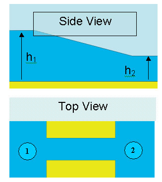
Basis of Investigation

Marine currents tend to develop in channels between land masses. Each channel is of course unique in terms of its width and depth variations, roughness etc. The idea was therefore to take a real channel and idealise it into a simple mathematical model. The basic assumptions made included;

• Flow in the channel originates from the out – of – phase rise and fall in two tidal reservoirs at the end of the channel.
• The reservoirs were considered to be large and therefore their rise and fall is independent of any flow in the channel.
• The effects of seabed topology on the flow velocities are neglected

Back to top

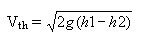
Procedure

Step 1:

Sea level data from two reservoirs on either end of the channel were obtained such that when the tidal height at the first reservoir is h1 the second h2 is out of phase by an angle Φ or at a different height. These heights were therefore expressed by a sine approximation given by the equations

H1 = H1Sinωt

H2 = H2Sin (ωt + Φ)

But this need not apply to all channels.

Step2:

The ideal (theoretical) velocity (Vth) is therefore estimated as

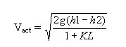
Step3:

This theoretical velocity is then compared with actual measured marine current velocity (Vact) of the channel to estimate an effective loss coefficient for the channel (KL)

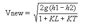
Step 4:

Effects of MCT’s

The effect of blockage is then investigated by installing marine current turbines (MCT) in the channel with a turbine coefficient KT. With KT known (representative of the number of turbines) and KL already found from step 3 above, the new channel velocity is estimated from

As KT increases (meaning more turbines), the channel velocity decreases.

The extractable power from the channel is directly proportional to KT and channel velocity and therefore it is expected that power will reach a maximum at some point.

Step 5:

Optimum KT

A trial and error method was used to find the KT value corresponding to maximum power. However for economical reasons, the optimum value of KT is not that value corresponding to maximum power but rather the value beyond which there is no significant increase in extractable power to justify the additional cost of turbines to be installed. This optimum KT value was found by finding the slopes to various points to the Power against KT curve. The optimum point is where the decrease in slope as compared to the slope at the beginning minimizes the power drop off. From our computations it is roughly about 60% presenting a power drop off of about 40%, which is more like a worse case scenario. For more optimist considerations, power drop off can be taken to between 10 – 20%.

Step 6:

How Many Turbines?

What does optimum KT represent in terms of number of turbines?

This was investigated by expressing solidity in terms of the turbine swept area.

Solidity, σ = Σ MCT Rotor Areas/Area of Channel

Betz analysis for wind turbines (and MCT’s) suggests that for maximum power extraction, the drag coefficient defined in

F D = C D* 1/2* ρ *A MCT * V 2 should be 8/9

It can be shown that in general KT = CD * σ and for maximum power σ = 9/8 KT

Thus the optimum solidity can then be found using KT estimated from step 5. The optimum solidity is then used to estimate the number of numbers that is equivalent to that blockage represented by KT from

Number of turbines = solidity * Area of Channel/MCT rotor area

Back to top