For an LCA to be exhaustive, according to our time for the project, we set some boundaries to work the LCA.

System boundaries that included in our study:

1. Raw material extraction and production of engineered materials

2. Manufacturing of building components

3. Transportation of materials from raw material extraction to part fabrication, and from there to building site.

4. Energy consumed during use phase of the building.

5. Embodied energy of replacement and maintenance materials

6. Efficiency factors will be used to cover manufacturing and construction losses for construction materials.

7. Lifespan of building will be assumed at 70 years.

System boundaries that omitted from study:

1. Furniture, floor carpet, windows frames, cleaning materials, paints, he electrical equipments, such as projectors, lighting, bulbs, phones, The switches and the sockets, cable terminals boards, etc.

2. Indoors air quality issues (off-gassing from paints and flooring and cleaning materials)

3. Energy consumption related to treating/supplying water and waste treatment

4. Energy consumption related to pick up and disposal of municipal solid waste

5. Methods and equipment used in construction phase

6. Environmental and social issues related to the origin of construction materials (effects on local economy and resource use)

7. Future technological breakthroughs that may have an impact on the LCA

8. For the transportation of the materials we did not get into account the energy required by the driver in order to get the materials to construction, to assembly, to replacement point and finally to elimination phase which consist of the recycling, incineration and landfill point.

In order to assess the LCIA, we required some impact factors on which to base our analysis. The ISO stds for LCA do not provide impact factors on which to judge the LCIA, however from the literature review it was decided that the most appropriate impact factors were contained in the CML methodology. These were:

1. Global Warming Potential – this is the effectiveness of a compound in contributing to global warming on a molecule-by-molecule basis measured relative to CO2.

2. Acidification Potential - The acidification potential is calculated for each material relative to 1kg of Sox.

3. Photochemical Ozone Creation Potential or (POCP) – Photochemical ozone creation measures the potential of emissions to air to form harmful ground level ozone, a precursor to smog.

4. Non renewable energy – This is the amount of energy required that comes from a non-renewable source. Non Renewable Energy is different to embodied energy, as embodied energy takes account of the energy that comes from both renewable and non-renewable sources.

In order to carry out an LCA analysis, we first had to find a suitable building for using as a case study within our project. This required detailed records of the materials of construction, with an inventory breakdown of the required amounts of each material within the building construction. After consultation with various contacts, including architectural firms, university lecturers and post-graduate students, we finally decided on using the plans for a school in Glasgow, which had previously been studied by one of the post-graduate students within the university and which an ESP-r model had been constructed. The reason for using this building was that the LCA is a very complex process and by using this model, we were able to obtain a full material inventory breakdown and also model the energy use of the building which would otherwise have been very difficult to achieve in the project time-frame. In order to simplify the LCA further, we chose one classroom from the model on which to base our LCA study. Through consultation with an electrician, we were able to produce a wiring diagram of this room and also carry out an LCA on the wiring system, which will be explained later.

A diagram of the ESP-r model of the classroom is shown below with each part of the room labelled:

The total manufactured mass of construction material may not necessarily be equal to the material mass used to construct the room, due to losses occurring in the manufacturing stage, transportation stage and construction stage.

Using the data from the ESP-r model, we were able to obtain the required construction mass of each building material.

Volume of each material = Thickness x Surface Area

Mass of material = Volume x Density

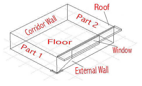
 All calculated material masses are shown in Figure 1

NB/ the materials of construction are shown as they appear in the ESP-r model for simplification. Notice that for each room portion, there appears to be some materials mentioned twice. This is a function of the ESP-r model, which is required for accuracy, as the material is divided into several parts due to the position of the nodal points within the software. Both portions account for the total material usage.

However, as stated previously, the construction mass for the building incorporated all the losses mentioned previously (manufacturing, transportation, construction). In order to calculate the total manufactured mass, we must obtain data of the expected losses during manufacturing, transportation and construction of each of the materials within the classroom. This data has been taken from previously published data.

Calculating the total manufactured mass of material, incorporating all the expected losses is an iterative procedure working in reverse order from manufacture. The transport losses to the construction point should be calculated first, then the transport losses to the pre-fabrication point (if required) should be taken into account. As can be seen from Figure 2, only the window is a pre-fabricated unit, which requires transportation distances from pre-fab site to construction site. Finally, losses in the manufacturing phase should be accounted for. What has not been mentioned is that each construction material has a finite lifespan, which may be less than the classroom lifespan. If we look at mineral fibre as an example, the expected lifespan of this material is 30 years. If we carry out the LCA over a period of 70 years, then this would require at least 2 replacements of this mineral fibre, one after 30 years and another after 60 years. In practice this would be unlikely due to the fact that the second replacement would probably not occur, since the building will be decommissioned only 10years after the replacement. If we look at this in numerical terms:  

Building lifespan = 70years

Material lifespan = 30 years

No. of material loads of mineral fibre = 70/30 = 2.3333

In practice the effective number of times that a material is replaced in a real building corresponds to a round number (integer). Therefore, we have assumed that the no. of material loads will be rounded to the nearest integer, which gives us the number of replacements over the building lifespan.

Therefore the number of material loads of mineral fibre required will be (2.3333), rounded to the nearest integer = 2.

Transportation also has a value associated to each of the impact factors, by which we are assessing our LCA, depending on the vehicle size and type.

In order to calculate the impacts associated with the transportation of each material, the manufacturer of each building material must be known. At this stage however, due to the fact that we did not have a bill of materials from the actual building, we had to make a best approximation of the material manufacturers, and we did this by visiting various building material merchants to find the most popular manufacturers for each construction material. This allowed us to estimate the manufacturer and the distance from the manufacturing point to the construction site.

In order to accurately assess the transportation impacts associated with construction of the building, the vehicle types must be known also. Again, this level of detail was unavailable to us, therefore as a best approximation, we used the same modes of transport for each material as had been used previously in a PhD research study for a building constructed in Switzerland. The two types of transport required for material transportation for the materials used in the classroom construction, were a 16ton lorry and a 26ton lorry.

When examining the manufacturing process of the construction materials, each material has a value associated to the impact factors that we have chosen for doing our LCA study. The manufacturing impacts for all the construction materials are shown in Figure 5. These impacts take into account raw material extraction, transportation of raw material to extraction point and the energy used in the manufacturing process.

When examining the transportation of the construction materials, each transportation type has a value associated to the impact factors that we have chosen for doing our LCA study. Two types of transportation were identified as being inclusive within our study - transportation from 16 ton and 28 ton lorries. The impact values associated to these two types of transport are shown in Figure 7.

NB/ the impacts are related to tons x km of material. Therefore in order to calculate the total transportation impact of each material, we must multiply these impact values by the total manufactured mass of each material and the distance that is travelled in km (refer to figure 4). This gives us the total transportation impacts as shown in Figure 8.

In order to calculate the energy required during the use-phase of the building, we ran the ESP-r model to obtain the Joules required throughout one year. This value was multiplied by the assumed building lifespan (70 years), to obtain the total energy required throughout the life span of the building.

We found that the total energy required for the classroom throughout the life span of the building was 2.828E+06 MJ. In order to assess the total impacts of the energy used within the building, we required impact values for the electricity (we have assumed that the total energy used will be from an electricity source. Within the classroom, this may not be strictly true, however electricity produces the highest impacts per MJ used, so this will produce a worst-case estimate). The impact factors for electricity produced within the European union are shown in Figure 9. (These figures represent the impacts per MJ of electricity used which account for both the production and use of the electricity).

The calculations for the Elimination phase of the building are based on a similar principle to those carried out for the pre-use phase. The disposal processes for each construction material (whether it be landfill, incineration, or recycling) have a value associated with each of the impact factors mentioned previously. The disposal method of each construction material requires to be known with corresponding transport distances to the disposal point. Quantifiable values for the elimination phase are very difficult to obtain so as a best approximation, we referred to a study carried out on a previous building assuming the same elimination phase values, but making a best approximation of the transport distances to the points of disposal. These are shown in Figure 11.

As can be seen from Figure 11, there are 3 variations in the waste disposal processes of all the building materials, which were recycling, incineration and landfill.

Each of the disposal processes has both an associated transport impact and disposal impact. The transport impacts were calculated as shown previous (refer to Figure 7). Each of the disposal processes has a value associated with the impact factors chosen for carrying out the assessment. These are shown in Figure 12.

Having carried out all calculations as listed above, this gave us quantifiable values for impacts associated to each of the three phases of the building i.e. pre-use, use and elimination phases, which could be compared to show how much environmental impact each phase accounted for. The results are plotted in graphs shown below:

1. Total Non Renewable Energy Impacts

2. Total Global Warming Potential Impacts

3. Total Acidification Potential Impacts

4. Total Photo-Chemical Ozone Creation Potential

The products we choose were from the Pirelli cables. For the room we estimated after the help of an electrician that we are gone use four types of cables.

a)      Lighting circuit – 6241Y/6242Y/6243Y to BS 6004

2-core cable of 1.5/1.0 phase/cpc dia 4.7*8.2 mm

b)      Electrical ring circuit - 6241Y/6242Y/6243Y to BS 6004

2-core cable of 2.5/1.0 phase/cpc dia 5.3*9.9 mm

c)      Emergency lighting - 6241Y/6242Y/6243Y to BS 6004

2-core cable of 1.0/1.0 phase/cpc dia 4.7*8.2 mm

d)      Smoke alarm – FP200 Flex to BS 6387

2-core cable 1.5 csa dia 8.2mm

The design life of the above products is a minimum of 20 years, but we expect that in reality it would be greater than 30 to 40 years.

Most 1.0mm2 and 1.5mm2 cables in houses have either a 5 or 6 amp fuse attached.

Most 2.5mm2 cable is used in ring circuits and have either 30 or 32 amps fuse attached.

Then we estimated the meters of each type of the cable that will be used in a room of 69.7 mm².

a)      Lighting ring – 22m for 6 ceiling lights evenly placed on the ceiling and exiting through the ceiling.

b)      Electrical socket ring – 40m for 2 sockets on each wall and circling the room in a main ring and leaving through the ceiling.

c)      Emergency lighting – 10m for 2 emergency lights placed centrally in the ceiling.

Pirelli can supply a full range of low voltage building wire products, which are commonly used in construction wiring. PVC, AFUMEX and Fire Performance product ranges are available, tailored to meet the requirements of national markets around the world. Our building wire products are manufactured and tested in accordance with international harmonised standards or local specifications.

In the following the products are described.

The environmental impacts have been studied for the three main phases of the cable system life cycle.

1. The manufacturing phase is the phase where the cables system is manufactured at Pirelli Company.

2. The use phase is the phase when the cables system is used at the customer. The most important environmental impact here is the losses of energy.

3. The disposal phase is the phase when the cable system is terminated in its use and is scrapped.

After we choose the type of cable that we are gone use, the next step was to find for each one of them the different materials that included in each cable Figure 17.

With the help of Pirelli we find the proportion of each materials weight for 1 km cable and multiplied it with our known length for each cable.

By also knowing that the design life of the cables was 35 years and our life cycle analysis was for 70 we took the decision to replace once all the cables in the room and so with this we found the total mass that we are gone use for a lifetime of 70 years. Also an assembly loss of 3% was calculated for all the materials. 

Example: Lighting circuit- PVC

The next step was to assess the impact that the cables material weight will have on the environment. By using the four indicators (NRE, GWP, AP, POCP) we could calculate the total impact to the environment during the manufacturing process for each one of the cables Figure 18

Example: Lighting circuit- PVC

Before calculate the use phase of the cables we had first to find the impact in transporting the cables from the manufacturing site to our school. Even though that the total mass of the cables was extremely low we used as a transport mean a lorry of 16 tonnes and this because we wanted to have as much as we could accurate results. The distance from the manufacturing site was obtained by taking consider the Pirellis factory in Hampshire. The impact values for the transport mean were taken from the same databases as for the materials see Figure 19.

Example: Lighting circuit

For the use phase we calculated the total energy losses in cables for the time of 70 years. From the known cables we knew the conductor resistance for 1 km and the current that pass through the wires. From these two we could calculate the energy loss of a cable for a length of 1 km, by using the type of P = I2*R. From the extracted numbers we were multiplied them with the total time (in sec) in a period of 70 years to get the total energy losses. Because the room was a school class the using of the power all day for 70 years wasn’t correct, so we multiplied it with a correction factor of 0,7 to have better results. From the database we found the impact for the consumption of energy that was calculated by taking the indicator values for the UCPTE see Figure 20.

Example: Lighting circuit

The last step was to calculate the impact of the cables during the disposal phase see Figure 21. So in this stage first we estimate the impact of the transport to the landfill site and after the impact that the waste will have on the environment. We decided to find the impact for the landfill site and not for the recycling or the incineration because is more common after the use of the cables to through them in the landfill and not separate each material to recycle it or incinerate it see Figure 22. Because we didn’t had the information that we needed to calculate the impact of the waste we forced to use from the database a common factor (Inerte waste) for all the materials so the final results aren’t as accurate as we would like see Figure 23.

Example: Lighting circuit

To find the transport impact we followed the same steps as previously mentioned in the “transport impact” table. The difference was only in the distance from the school to the landfill. Our new distance was 100 km including the return of the lorries. So the new tkm unit was 0,375703 tkm and the total impact NRE = 2,190E+00, GWP = 1,395E-01, AP = 1,204E-03, POCP = 1,242E-03.

After we finished the calculation of the environmental impact for all the three phases together with the transportation stages we gather all the results in one table to compare the stages for each indicator between them. From the boundary definition we decided that the two transport processes would be added in the manufacturing and in the disposal phase respectively. By observing the results through the use of graphs we can see that in the indicators of NRE and GWP the manufacturing and the use phase are the most important stages. The NRE shows as that the largest amount of energy consumed is for the manufacture of the product and in the use and also that these two extract the largest amount of CO2 in the atmosphere something that harms the environment. In the AP and POCP indicators the manufacture phase seems to be the main responsible for extracting substances such as SOx and C2H4. Also we can see the negligible impact that the elimination phase has in the four measured indicators.

In order the results of the impacts to be clearly for the audients, we produce graphs for each impact factors, of a comparison of the Building impacts with the Cables impacts. when considering the impact of the wiring compare with the overall building it can bee seen that the impacts are very small.
The Non Renewable Energy Impacts for the building pre-use phase are 4.096E+05MJ and for the cables pre use phase are 1.829E+03MJ. The impacts for the building use phase are 1.005E+07MJ and for the cable use phase are 1.780E+03MJ as we can see the cables impact on that phase are negligible according to the building impacts. The impacts for the building elimination phase are 2.567E+04MJ and for the cables elimination are 1.112E+01MJ.
For the Global Warming Potential Impacts we followed the same procedure in order to calculate the impacts for the building pre-use phase which are 2.775E+04Kg CO₂-equiv. and for the cables pre use phase which are E9.475+01Kg CO₂-equiv.. The impacts for the building use phase are 4.754E+05Kg CO₂-equiv. and for the cable use phase are 8.416E+01Kg CO₂-equiv.. As we can see there is an incensement of the impact in that phase than the previous one because we are taking into account the life span cycle years which is 70 years. The impacts for the building elimination phase are 3.520E+03Kg CO₂-equiv. and for the cables elimination are 7.108E-01Kg CO₂-equiv.

For the Acidification Potential impacts as shown on the table below the impact for the building pre use phase is 1.539E+02Kg SOx-equiv and for the cables at that phase are1.492E+00Kg SOx-equiv. At the at the use phase of the building the impacts are 3.396E+03Kg SOx-equiv and the cables are 6.013E-01Kg SOx-equiv. For the elimination phase the results we got were: for the building 1.594E+01Kg SOx-equiv and for the cables 6.143-03Kg SOx-equiv.

Finally for Photochemical Ozone Potential we got that the impacts for the pre use phase of the building

are 1.103E+01Kg C2H4-equiv.+NOx and for the cables are 2.438E+01Kg C2H4-equiv.+NOx. Also for the use phase of the building the impacts are 6.903E+02Kg C2H4-equiv.+NOx and for the cables are 1.222E-01Kg C2H4-equiv.+NOx. At last the impacts of the elimination phase of the building are 1.487E+01Kg C2H4-equiv.+NOx and for the cables are 6.3455E-03Kg C2H4-equiv.+NOx which is almost negligible. 

The impact associated with the photochemical ozone potential for the cables, produces slightly higher results than for the other impact factors. In numerical values, the cables accounted for approximately 3% of the total POCP impacts. It should be noted however that due to time constraints, we did not take account of bulb replacement in the lighting circuit, or fuse resplacement for all circuits which would have an increased impact on the wiring system.