Uncertainty

Simulation models are abstractions of designs which, when processed by numerical engines, give rise to predictions which appear to be precise. Such reporting precision is probably unwarranted. Building are rarely implemented exactly as the construction documents specify, materials properties may differ between batches, thermostats may be poorly calibrated, ducts and fans may not have been properly comissioned. The way a building is used and the number of occupants may only roughly correspond to the assumptions used in the design process.

The abstraction needed when translating designs into the descriptive syntax of simulation tools introduces risk in the form of approximations and input errors. It is thus useful to explore whether variability in the form and fabric and use would lead to different design decisions or to the management of facilities. There are many approaches users can take to introduce uncertainty into models:

Manual interventions - users can hack the model description files. This is often deceptively easy and just as often difficult to manage. It presumes a knowledge of the location and syntax of model entities as well as numerical skills needed if the aim is to implement a formal uncertainty regime. The user then comissions assessments, extracts performance data and then repeats the exercise (perhaps with some automation).

Bespoke agent-based interventions - software agents with an embedeed knowledge of the location and syntax of model entitie and drivers for uncertainty regimes are used to automate the process of peturbing the model, invoking the required assessments and undertaking performance data extraction. Here the agent is bespoke (i.e. designed to implement specific uncertainty regimes on a specific model).

Embedded formal interventions - uncertainty directives are part of the model description and acted upon by the simulation engine, perhaps with a managing agent that is also taking its instructions from the formal uncertainty directives found in the model.

There are, of course, any number of ways to impose changes within a simulation model - a) users can manually drive the simulation tool interface (this does not scale well), b) a pattern matching language such as grep can be used to search and replace tokens in the model files, c) scripts can drive the tool interface to carry out specific editing tasks.

Uncertainty explorations may involve the creation of scores, if not hundreds, of model variants. Proving that the process is robust is one of many challenges. Few simulation tools were initially designed to accommodate large numbers of models and the skills used to support normal simulation use differ from those needed to manage a diversity of models.

ESP-r approach

Any of the above approaches can be used with ESP-r. It's interface can be driven via scripts, inbuilt editing facilities will support most attribute changes, the model description files are ASCII and can thus be edited by a variety of methods or subjected to pattern matching interventions and the data model includes formal descriptions of uncertainty.

We will focus on the embedded formal intervention approach within ESP-r. It uses a formal description of uncertainty which takes the general form of named lists of what attributes of the model are uncertain and named lists defining where (temporal scope or location). These What/Where defintions are paired as needed. The attributes of a model which can be uncertain include thermophysical properties, surface properties, zone casual gains, ideal controls and weather data:

thermophysical properties of a material - conductivity, density, specific heat, surface emissivity and absorptivity and diffusion resistance

layer thickness within construction,

zone air volume or a surface area,

weather data - dry-bulb temperature, direct normal & diffuse solar radiation, wind speed and wind direction, relative humidity

zone operations attributes for scheduled air flow - infiltration, ventilation, ventilation source temperature

zone operations attributes for casual gains - sensible or latent magnitude, radiant or convective fraction, period start time

ideal zone controls attributes e.g. heating and cooling magnitudes, period start times,

The attributes of what-is-uncertain, for example user named definitions [wall_insul_thick] and [roof_insul_thick] identify a layer of insulation in two different constructions which might be used in various locations in the model. Each such definition also includes a range and/or bound of uncertainty, either as a % of the nominal value of the attribute or a fixed offset i.e. 0.02m. The Where definitions for construction uncertainties e.g. [facade_walls] and [the_roof] would include a list of associated surfaces. There are also options to define locations for all surfaces which use a specific MLC or material.

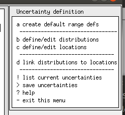
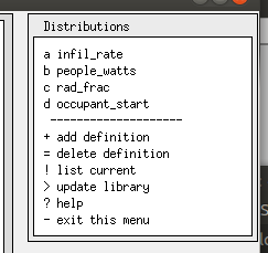
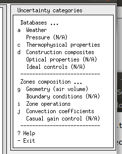
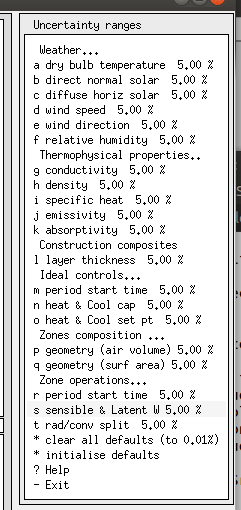
In the figure below the upper left is the main uncertainty menu, the center is the categories of model entities, the right are a list of current uncertainty ranges and the lower left are a set of user-named distributions.

When bps starts it recognises that there are uncertainty defintions and ask the user whether a differential, factorial or Monti-Carlo assessment should be used and how many runs should be comissioned, typically 50-100. All runs are held in the same results file as separate [results sets].

At the start of each run the model details are scanned and the uncertainty description drives the modification of the model attributes in memory (no model files are changed). A random number is generated (a standard distribution between -2 and +2) which is applied to each uncertainty concept and its range/bounds directives.

The results analysis facility recognises the uncertainty sets and enable a [sensitivity] menu which allows analysis within the full range of [results sets] or between specific sets.

The dialog when res starts might look like:

 The name (uncertain_ctl.res) will be used.
 Opening file with record length 40
 Databases scan (ok)
 Number of result-sets held = 20
 Set|Control    |Start |Finish| Time   | Save |Average|Pre|Aid memoire
 no.| name      | day  | day  |steps/hr|option| Flag  |sim|(for this set)
  1 float until   1, 2  28, 2       4      4       0   21  U01 0.42 U02 0.23
  2 float until   1, 2  28, 2       4      4       0   21  U01 0.81 U02-1.07
  3 float until   1, 2  28, 2       4      4       0   21  U01 0.57 U02 2.25
  4 float until   1, 2  28, 2       4      4       0   21  U01-0.77 U02 1.64
  5 float until   1, 2  28, 2       4      4       0   21  U01-0.66 U02 0.07
  6 float until   1, 2  28, 2       4      4       0   21  U01 0.81 U02-0.04
  7 float until   1, 2  28, 2       4      4       0   21  U01-0.05 U02-0.90
  8 float until   1, 2  28, 2       4      4       0   21  U01-0.89 U02-0.21
  9 float until   1, 2  28, 2       4      4       0   21  U01-1.93 U02 1.37
 10 float until   1, 2  28, 2       4      4       0   21  U01-1.23 U02 0.06
 11 float until   1, 2  28, 2       4      4       0   21  U01 0.52 U02 0.17
 12 float until   1, 2  28, 2       4      4       0   21  U01-1.20 U02-1.82
 13 float until   1, 2  28, 2       4      4       0   21  U01-0.28 U02-0.01
 14 float until   1, 2  28, 2       4      4       0   21  U01 1.75 U02 1.57
 15 float until   1, 2  28, 2       4      4       0   21  U01-0.64 U02-1.08
 16 float until   1, 2  28, 2       4      4       0   21  U01 0.52 U02-1.28
 17 float until   1, 2  28, 2       4      4       0   21  U01 0.23 U02 1.06
 18 float until   1, 2  28, 2       4      4       0   21  U01 0.64 U02-0.16
 19 float until   1, 2  28, 2       4      4       0   21  U01-0.52 U02-0.50
 20 float until   1, 2  28, 2       4      4       0   21  M-C run:  19
The current result library holds data from a monte carlo uncertainty analysis
 Do you wish to analyse:  a) the uncertainties, b) a particular set ? 
 . . .

Below is a tabular list of inter-set statistics:

Zone db temperature (degC) is focus
room is focus
  Hour      Maximum       Minimum        Mean          Standard
             value         value         value         deviation
  0.12       13.7494       12.8298       13.2896        0.4598
  0.38       13.6880       12.7798       13.2339        0.4541
  0.62       13.6325       12.7358       13.1842        0.4483
  0.88       13.5800       12.6946       13.1373        0.4427
  1.12       13.5243       12.6499       13.0871        0.4372
  1.38       13.4583       12.5944       13.0264        0.4319
  1.62       13.3858       12.5319       12.9589        0.4270
  1.88       13.3125       12.4682       12.8904        0.4222
  2.12       13.2418       12.4068       12.8243        0.4175
  2.38       13.1771       12.3514       12.7642        0.4128
  2.62       13.1166       12.3002       12.7084        0.4082
  2.88       13.0575       12.2503       12.6539        0.4036
  3.12       12.9997       12.2015       12.6006        0.3991
 . . .

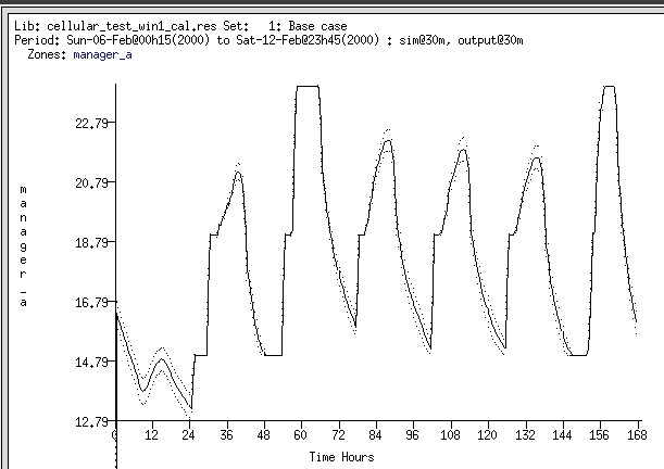
There are also options for colum listings of timestep values for each of the simulation sets for most of the preformance metrics within the performance file. A graphic view of the distribution of zone dry bulb temperatures over time is shown below: