Simulation speed
© Copyright 2018 Energy Systems Research Unit, Glasgow, Scotland

|
Those who use simulation tools are familiar with
waiting for the kettle to boil. Unlike the impatient
cook, simulation users can actually influence the resources required
to carry out tasks -- if we understand the resource implications
in how we design our simulation models, the workflows we use and the
bottlenecks within our computing platforms. Improvements of an
order of magnitude in specific tasks are possible.
The method used to highlight these opportunities is the creation of a test matrix which includes simulation models at various levels of complexity, various assessment goals, various simulation frequencies and performance-data-to-save directives, computational rigour directives across a mix of legacy and current computing platforms, operating systems. And just to spice it up we will look at the implications of the tool chains used to build simulation tools and run alternative simulation tools across the matrix. |
What we found:
User choice implications
What we choose to include in our virtual worlds of physics and our design decisions within those virtual worlds have consequences. Although simulation tools may guide (or coerce) us, decisions about the extent of our models and the levels of detail it contains is ultimately down to the model design decisions of practitioners. Following the easy path though the tool does not necessarily create a model which is fit-for-purpose. Enough said. The benchmarking matrix includes two models. The first is a pair of cellular offices with a corridor. Its composition and complexity characterises the exemplar training models distributed with simulation suites such as ESP-r and EnergyPlus. The second model was taken from a project on retrofit options for traditional heavy masonry apartments.
A simple training model
Models used for training in simulation tools tend to be constrained in complexity. Often training models have a half dozen zones, perhaps 40-50 surfaces and straightforward environmental controls. Such model constraints reflect novices abilities and, in general, assessment tasks associated with them make minimal demands on computers.
|
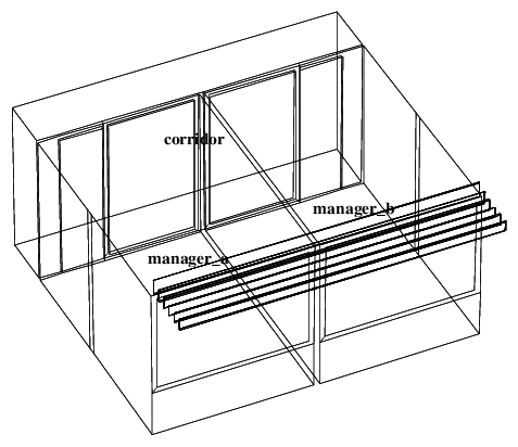
The figure to the left is a training model distributed with ESP-r.
It has two identical cellular offices with a corridor. Glazing frames are
separate surfaces and some of the walls have been subdivided.
This model was also exported as an EnergyPlus IDF file V8.8 so the assessment timings
are well matched in terms of the zones, surfaces, surface composition,
casual gains as well as startup days, assessment periods and timesteps.
However, to accommodate the Conduction Finite Difference solver in EnergyPlus (see grumble later on), the conductivity of steel in the floor structure was reduced and a fibre concret rainscreen was substituted for the standard metallic rainscreen in the facade. ESP-r uses a finite volume solver which is less sensitive to high conductivity materials (complaints start with layers of 0.4mm thickness). The contents of this model are reported in this ASCII contents file or as a PDF file |
The periods of assessment, timesteps, warmup periods and solar shading directives for the EnergyPlus model were also matched. Both 4 TSPH and 20 TSPH and both the CTF and CFD solvers are exercised in EnergyPlus and ESP-r uses its Finite Volume approach. One difference is the use of a free floating control for the EnergyPlus runs.
High-mass traditional apartment
Models which represent real buildings often explicitly represent most, if not all, of the rooms in the building as well as specific aspects of the building facade. They may also abstractly represent adjacent spaces which represent bounding conditions and they may also include a degree of diversity in the occupancy and casual gains within the spaces so as to capture the response characteristics of the building.
To assist our comparison with EnergyPlus 4 & 20 TSPH assessments have been run. Twenty TSPH yields an annual results file of over 21GB (full zone and surface energy balances). Although the ESP-r res module can handle this the pedantic nature of the post processing requests tends to thrash the disk, indeed the quantity of data written also impacts the speed of the simulation. As will be discussed in a later section, it is possible to request that performance data be saved at a lesser frequency and to write a subset of data to the file. The latter technique has been used for the summer and annual 20 TSPH runs performance data was saved once per hour than at each timestep. User choices for recording performance data which impact on the size of the files are also explored. In a later section we will look at the implications across a range of user directives.
As with the simple office model the traditional apartment was exported to EnergyPlus version 8.8. Give the mass of the structure the Conduction Finite Difference solver is the solver of choice (the CTF solver is also tested). In this model only one instance of steel needed its conductivity relaxed to avoid a severe error. Again the assessment was run with a free floating control.
|
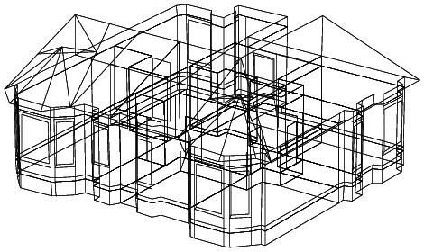
For this study we will use an 1890s
apartment in a sandstone building. Such models often represent each
room explicitly as well as the bay windows in the facade and the
different thicknesses of stone (up to 900mm thick). In this case
there are 13 zones and 432 surfaces. Environmental controls involve
radiators (mixed convection & radiation) with TRV (mixed sensors).
The figure below shows a view (including an abstract bounding zone
below the occupied space as well as the roof space above). The
usual range of timesteps for this model is 8-10 TSPH (there is
nothing in the model or the goals of the project which demands
a shorter timestep).
The contents of this model are reported in this ASCII contents file or as a PDF file |
Directives on simulation frequency
Our choices on assessment timestep is typically a compromise between the response characteristics of the building and its environmental controls, the what-do-we-need-to-record in order to confirm the design works and the constraints of the solver being used. In the matrix we use both a 15 minute timestep and a 3 minute timestep. Both tools support a minute timestep for the building solver and ESP-r can simulate plant at a fraction of a second although the latter is not explored in this study.
Ideally the timestep reflects either the frequency at which we want to explore performance issues or an aspect of an environmental control or mass flow which might undergo rapid changes.
Some solvers constrain the simulation timesteps - in the tables below the CTF method in EnergyPlus does not like frequencies less than 4 per hour (not sure about frequencies greater than 30 per hour). Most example IDF files use 4 or 6 timesteps per hour. The Finite difference method does not allow frequencies less than 20 per hour (20 30 or 60 are possible).
The extent and frequency of performance data captured during an assessment forms another matrix to explore. ESP-r has a concept of save levels two of which are explored - a full set of performance data (i.e. full energy balances at zones and surfaces) and a subset of performance data. The tests include both save levels and for longer periods a data frequency of hourly as well as each timestep. Post-processing in ESp-r recovers the following performance data for each zone:
The EPP assessment writes hourly data on:
as csv and ESO files but no further post-processing. These directives would need to be considerably extended to be comparable with what ESP-r stores. There is also no direct equivalent of the ESP-r res module so the method for comparing post-processing timings needs to be evolved.
To test the impact of writing data at higher frequencies (see disk-bound section below) variant IDF files were created with timestep directives.
Directives on simulation periods
To highlight the costs of uncritical generation of annual performance indicators and focused reality checks to gain confidence in models we include in the matrix the following assessment periods:
Pre-processing directives matrix
Directives which impose additional resolution on models, for example, computing surface-to-surface viewfactors, shading & insolation directives are computed prior to assessments and the stored results used during assessment.
Simulation tools offer a range of user directives for radiation exchange within zones. The process of computing and using surface-to-surface view factors in ESP-r is straightforward and seems to be where dragons live for EnergyPlus. In ESP-r the method is based on creating a grid of points on all surfaces. The grid resolution defaults to 10x10 per surface but can be increased (e.g. to cope with thin frames around doors and windows). Shifting to a ~40x40 grid would impact computing resources but is rarely required.
For ESP-r timings were taken on a Dell 7010 running Linux and ESP-r V12.7. The task of pre-computing surface-to-surface view factors rarely takes more than a minute and is often a matter of seconds. Pre-calculating the hourly distribution of solar insolation within a complex zone (including to the explicit mass surfaces) requires even fewer resources.
|
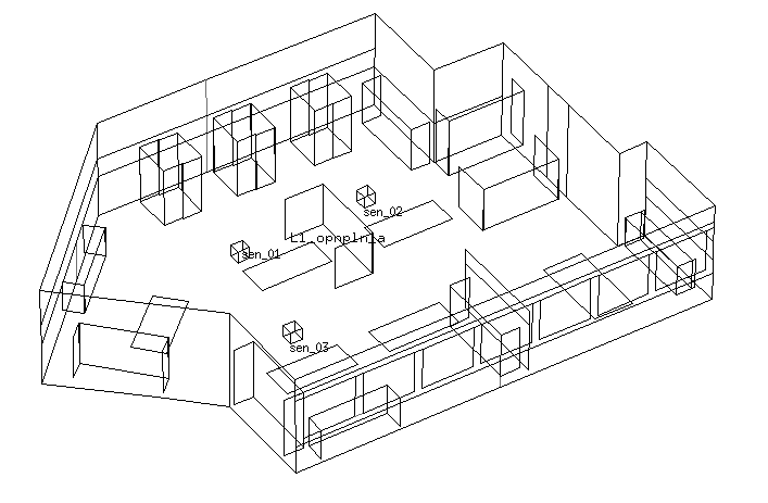
Two levels of romm complexity have been tested.
The room on the left includes 314 vertices, 152
surfaces of varying complexity from 4-36 edges in the facade as well
as dozens of explicit internal mass surface pairs representing
desks and filing cabinets.
Also seen are the location of MRT sensors (at occupant head locations for assessing radiant asymmetry). |
The pre-processing in the context of a simple zone (90 vertices 40 surfaces) such as that found in the simple pair of offices implies the following overhead:
In addition to the time taken for actual calculations the specification of user directives for shading and insolation requires a few seconds. There are a few options to set in terms of the accuracy of viewfactor calculations as well as locating and defining MRT sensor locations.
As zones evolve shading is automatically updated. If the location on site is adjusted all shading is automatically updated and because there is no user interaction needed it may take only a few seconds per zone. Viewfactor calculations require the user to initiate the calculations. In a 90 zone model this becomes a repetitive task that probably should be automated.
Assessment directives matrix
Simulation models include a range of directives which impact computing resources.
Hardware choices
Each computing platform includes a mix of hardware which can impact how much time the kettle takes to boil. Each epoch of computer has quirks as well as opportunities for fine tuning. And there are the disruptor platforms which may find application in some simulation scenarios.
Computer matrix
The following table describes the matrix of computers included. The columns are:
| Computer | CPU | CPU speed | memory | OS | tool-chain | disk type | comment |
|---|---|---|---|---|---|---|---|
| Dell 7010 | 4x Intel i5-3470 | 3.6 GHz | 8GB RAM | Ubuntu 16.04 | GCC 5.4 | rotational | 2013 epoch standard workstation |
| Dell 7010 | 4x Intel i5-3470 | 3.6 GHz | 8GB RAM | Windows 10 | GCC 5.4 | rotational | 2013 epoch standard workstation |
| Dell 7010 VirtualBox | 2x Intel i5-3470 | 3.6 GHz | 2.4GB RAM | Ubuntu 16.04 | GCC 4.8 | virtual disk | Non-commercial virtualisation with constrained RAM CPU & disk performance |
| Dell 7010 VMware | 2x Intel i5-3470 | 3.6 GHz | 2.4GB RAM | Ubuntu 16.04 | GCC 4.8 | virtual disk | Commercial virtualisation with constrained RAM CPU & disk performance |
| Dell 780 | 2xIntel Core2 Duo E8400 | 3.0 GHz | 4GB RAM | Ubuntu 16.04 | GCC 5.4 | rotational | 2010 epoch typical of legacy kit |
| MacBook Pro (2012) | 2x Intel i5 | 2.5 GHz | 8GB RAM | OSX 10.10.5 | GCC 5.3 | SSD | Typical legacy OSX laptop |
| MacBook Air (2013) | Intel i5 | 1.3 GHz | 4GB RAM | OSX 10.13.0 | GCC 6.3 | SSD | Fast SSD and memory, faster than GHz would indicate |
| Odroid C2 | AArch64 | 1.53 GHz | 1.8GB RAM | Ubuntu 16.04 | GCC 4.9 | SDHC | One of the more powerful ARM SBC |
| Pinebook64 | AArch64 | 1.34 GHz | 2GB RAM | Ubuntu Mate | GCC 5.4 | emmc | ARM based Laptop with EMMC disk |
| Raspberry Pi3 | ARMv71 | 1.2 GHz | 1GB RAM | Debian 8 | GCC 4.9 | SDHC & rotational | Popular ARM SBC hosted on a rotational disk. Memory constrains the complexity of models that can be hosted. |
Timings for a simple training model
In this table the assessment times are shown for ESP-r V12.7 compiled with no optimisation and high optimisation with the GCC tool chain on all computing platforms. Where EPP V8.8 was locally compiled the same compiler and optimisation levels were used. For Windows 10 the EPP suite was a pre-compiled download.
This particular ESP-r model is normally run at 4 TSPH, however the CFD solver in EnergyPlus requires at least 20 TSPH so ESP-r runs were made at both 4 and 20 timesteps per hour.
In the table below times are in seconds use the syntax for ESP-r is (4tsph simulation/reporting) [20tsph simulation/reporting] and for EnergyPlus is (CTF conduction transfer function simulation & ReadVars) [CFD conduction finite difference & ReadVars].
| Platform | Suite | One week | Jan-Feb | Summer | Annual |
|---|---|---|---|---|---|
| Dell 7010 Linux Ubuntu | ESP-r optimized | (<1 <1) [2 <1] | (2 1) [6 2] | (3 1) [11 4] | (7 3) [30 10] |
| ESP-r un-optimized | (1 <1) [4 <1] | (3 1) [12 2] | (5 2 ) [22 5] | (13 5) [59 13] | |
| EPP downloaded | (1 <1) [4 <1] | (2 <1) [11 <1] | (3 <1) [19 <1] | (7 1) [52 1] | |
| EPP local optimized build | (1 <1) [3 <1] | (2 <1) [11 <1] | (3 <1) [19 <1] | (7 1) [53 1] | |
| EPP local un-optimized build | (2 <1) [13 <1] | (5 <1) [41 <1] | (8 <1) [72 <1] | (22 1) [199 1] | |
| Dell 7010 Windows 10 | ESP-r optimized | (2 1) [2 2] | (3 1) [8 9] | (4 3) [14 16] | (8 10) [34 49] |
| EPP downloaded | (1 <1) [4 <1] | (2 <1) [9 <1] | (4 1) [17 1] | (8 3) [47 3] | |
| Dell 7010 VirtualBox Linux | ESP-r optimized | (2 <1) [3 1] | (3 1) [10 2] | (5 2) [17 7] | (10 5) [46 20] |
| EPP optimized | (<1 <1) [4 <1] | (2 <1) [11 <1] | (3 <1) [20 <1] | (8 1) [55 2] | Dell 7010 VMware Linux | ESP-r optimized | (2 1) [3 1] | (3 1) [11 4] | (5 2) [18 8] | (10 5) [45 28] |
| EPP optimized | (1 <1) [4 <1] | (2 <1) [11 <1] | (3 <1) [20 <1] | (8 1) [56 1] | |
| Dell 780 Linux | ESP-r optimized | (1 <1) [3 1] | (2 1) [8 3] | (3 2) [15 5] | (8 4) [40 13] |
| EPP optimized | (1 <1) [5 <1] | (3 <1) [16 <1] | (4 <1) [29 <1] | (11 2) [80 2] | |
| MacBook Pro | ESP-r optimized | (1 <1) [4 1] | (2 1) [9 7] | (5 3) [15 13] | (9 9) [38 28] |
| EPP optimized | (1 <1) [4 <1] | (2 <1) [12 <1] | (4 1) [25 1] | (9 2) [59 2] | |
| Odroid C2 | ESP-r optimized | (6 2) [16 5] | (13 7) [61 24] | (22 18) [117 47] | (66 32) [320 322] |
| EPP optimized | (5 <1) [16 <1] | (15 1) [97 1] | (29 3) [185 3] | (73 8) [539 8] | |
| Pinebook64 | ESP-r optimized | (7 4) [23 5] | (17 6) [74 15] | (41 11) [178 26] | (98 22) [378 72] |
| EPP optimized | (9 <1) [51 <1] | (24 2) [164 2] | (42 3) [300 3] | (113 10) [826 10] | |
| Raspberry Pi3 | ESP-r optimized | (6 4) [20 5] | (14 7) [63 20] | (26 12) [116 39] | (68 28) [320 137] |
| ESP-r un-optimized | (15 5) [61 8] | (40 14) [189 41] | (72 25) [346 95] | (197 68) [968 995] | |
| EPP optimized | (11 <1) [45 <1] | (21 2) [83 2] | (36 3) [248 3] | (95 10) [701 10] | |
| EPP un-optimized | (21 <1) [155 <1] | (55 2) [483 2] | (94 3) [849 3] | (246 9) [2390 10] |
Discussion
The table indicates that reality-check runs are in the order of seconds and seasonal/annual assessment tasks of one minute or less across most of the matrix of computing platforms. Unless you are undertaking automated parameter excursions the interactive user experience is little changed across the matrix.
At this scale there is no need to use the legacy EnergyPlus CTF solver (unless you are running on one of the single board computers or running longer assessments on legacy kit).
Windows shows a disadvantage for disk intensive activities. The EnergyPlus downloaded executables on Windows have an advantage over locally compiled Linux versions.
There appears to be little difference between the performance of non-commercial and commercial virtual computers for simple models. Indeed, at this scale of model there is little or no increase in assessment times in comparison with native tool performance (even with constrained memory).
For summer and annual assessments the use of un-optimized simulation tools shows a significant increase in timings. Essentially one would avoid un-optimized builds for production work, especially with models with any level of complexity.
Timings for the High-mass traditional apartment
In the table below times are in seconds use the syntax for ESP-r is (4tsph simulation/reporting) [20tsph simulation/reporting] and for EnergyPlus is (CTF conduction transfer function simulation & ReadVars) [CFD conduction finite difference & ReadVars]. A * indicates performance data generated at 20 TSPH but saved hourly.
| Platform | Suite | week | Jan-Feb | summer | annual |
|---|---|---|---|---|---|
| Dell 7010 Linux Ubuntu | ESP-r optimized | (11 2) [49 4] | (33 6) [156 33] | (59 12) [265 4*] | (166 33) [690 9*] |
| ESP-r un-optimized | (32 1) [147 2] | (94 4) [460 14] | (164 7) [793 3*] | (453 20) [2193 7*] | |
| EPP pre-compiled * | (3 <1) [51 <1] | (9 2) [153 2] | (17 4) [308 4] | (47 12) [791 12] | |
| EPP optimized * | (3 <1) [51 <1] | (9 2) [152 2] | (17 4) [315 4] | (46 12) [765 12] | |
| EPP un-optimized * | (11 <1) [207 <1] | (28 2) [605 2] | (54 4) [1243 4] | (142 12) [3080 13] | |
| Dell 7010 VirtualBox Linux | ESP-r optimized | (23 2) [109 5] | (73 3) [348 423] | (130 15) [595 5*] | (350 560) [1653 12*] |
| EPP optimized * | (4 <1) [58 <1] | (10 2) [168 2] | (20 4) [336 4] | (53 12) [974 12] | |
| Dell 7010 VMware Linux | ESP-r optimized | (25 2) [171 5] | (72 10) [335 214] | (122 16) [317 5*] | (304 260) [1392 13*] |
| EPP optimized * | (4 <1) [55 <1] | (11 2) [170 2] | (20 4) [407 4] | (54 13) [837 13] | Dell 7010 Windows 10 | ESP-r optimized | (12 4) [48 14] | (33 21) [157 108] | (58 43) [251 11*] | (158 126) [683 92*] |
| EPP downloaded * | (4 4) [49 1] | (11 4) [156 4] | (21 9) [297 9] | (58 26) [763 26] | |
| Dell 780 Linux | ESP-r optimized | (15 2) [74 7] | (49 11) [224 92] | (89 23) [366 6*] | (226 65) [1033 8*] ?? |
| EPP optimized * | (6 1) [90 1] | (13 3) [279 3] | (26 6) [529 6] | (69 20) [1392 18] | |
| MacBook Pro | ESP-r optimised | (4 2) [60 9] | (14 3) [197 86] | (76 66) [323 15*] | (195 36) [870 20*] |
| EPP pre-compiled * | (4 <1) [72 <1] | (13 3) [204 3] | (25 7) [404 7] | (67 20) [1028 23] | |
| Odroid C2 | ESP-r optimized | (134 9) [630 33] | (394 16) [1976 2172] | (775 328) [3455 24*] | (2171 2534) [9380 59*] | EPP optimized * | (34 2) [571 2] | (106 12) [1654 12] | (212 25) [3401 25] | (555 76) [8600 15] |
| Pinebook64 | ESP-r optimized | (193 6) [953 14] | (603 23) [3060 30] | (1119 44) [5121 15*] | (2899 128) [13852 36*] |
| EPP optimized * | (51 2) [825 2] | (160 15) [2378 15] | (308 32) [4887 32] | (822 35) [12316 35] | |
| Raspberry Pi3 | ESP-r optimized | (159 7) [754 20] | (457 34) [2269 222] | (831 91) [4185 20*] | (2294 304) [11484 67*] |
| EPP optimized * | (44 2) [724 2] | (131 15) [1862 15] | (253 32) [4155 32] | (638 34) [10351 34] |
Discussion
As the complexity of models increases different patterns emerge in the interplay between user directives and hardware.
Disk-bound assessments
Writing performance data and recovering it for inclusion in reports and graphs might be another elephant-in-the-room. The tests suggest a number of correlations with:
As seen in the above tables, simulation tasks via models such as the simple pair-of-offices are rarely disk-bound. The slow SDHC disks of some single board computers are somewhat impacted but with most legacy and current computers in the matrix users will hardly notice.
The table below illustrates the time implications in the context of the traditional apartment:
| Platform | Suite | Variant | Summer | Annual | Comment |
|---|---|---|---|---|---|
| Dell 7010 Linux Ubuntu (rotational drive) | ESP-r optimized | 20 TSPH-20 TSPH save everything | [288 145 elapsed ~7GB] | [787 2007 elapsed ~21GB] | Data recovery dependent on disk I/O, typically 50MB/s |
| - | 20 TSPH-20 TSHP save subset | [270 32 elapsed 590MB] | [731 96 elapsed 1.7GB] | Subset save reduces post-processing burden | |
| - | 20 TSPH -> 1 TSHP save everything | [266 4 elapsed ~350MB] | [727 10 elapsed ~1GB] | Data recovery minimal burden | |
| - | 20 TSPH -> 1 TSHP save subset | [264 2 29MB] | [727 6 88MB] | minimal gain from saving only a subset | |
| EnergyPlus | 20 TSPH -> 20 TSHP | [411 83] | [1087 248 ~6GB] | noticable post-processing resource | |
| - | 20 TSPH -> 1 TSHP | [312 4] | [793 12 ~310MB] | quick post-processing | |
| Macbook Pro (SSD) | ESP-r optimized | 20 TSPH-20 TSPH save everything | [387 1345] | [995 6036] | Data files ~21GB |
| - | 20 TSPH-20 TSHP save subset | [346 71] | [879 200] | Data files ~6GB | |
| - | 20 TSPH -> 1 TSHP save everything | [323 15] | [870 20] | Data files ~1GB | |
| EnergyPlus | 20 TSPH -> 20 TSHP | [563 12] | [1536 401] | Output folder ~6GB | |
| - | 20 TSPH -> 1 TSHP | [404 7] | [1028 22] | Output folder ~2GB | |
| Odroid C2 | ESP-r optimized | 20 TSPH-20 TSPH save everything | [- -] | [- -] | Not enough disk space. |
| - | 20 TSPH-20 TSHP save subset | [3392 249] | [9308 2866] | Data files ~6GB | |
| - | 20 TSPH -> 1 TSHP save everything | [3455 23] | [9380 59] | Data files ~1GB | |
| EnergyPlus | 20 TSPH -> 20 TSHP | [- -] | [- -] | Not enough disk space. A common limitation for ARM computers as well as virtual computers | |
| - | 20 TSPH -> 1 TSHP | [3414 25] | [8649 74] | Output folder ~1GB |
As models approach the complexity of the traditional apartment instances of disk-bound assessment begin to be noticeable, in some cases they begin to dominate. Where data recovery agent requests are supplied via the memory buffer tasks can be accomplished one or two magnitudes quicker. What we notice is that for disk writing from the simulation engine in ESP-r is roughly 10-50MB/second while disk reads, especially from large data stores might be half that speed. Where post-processing can take advantage of the operating system file buffers the data recovery is one or two orders of magnitude faster. Remember, writing of performance data is essentially a sequential task while post-processing of multiple topics can involve random access into the performance access if not multiple passes over the data store to derive statistics and/or generate graphs.
Although it does not show up in the graph, response to user interactions for non-simulation tasks are impacted, especially during post-processing. Pointers would freeze and simple tasks like folder listings could be an order of magnitude slower. Multiple processors may speed automated tasks but the user experience is degraded.
Users have a number of choices:
Workflows
The ordering of simulation tasks can have a substantial impact. Assessments which generate a large performance data sets and which are immediately followed by data recovery actions tend to be more efficient than running a series of assessments followed by a sequence of data recovery tasks.
On most computing platforms, even those with multiple processors, users will notice sluggish response for tasks carried out at the same time as heavy disk activity. To explore this consider the table below which looks at the time required for sequential and parallel simulation tasks.
| Computer | Period | Sequential sim | Sequential post-processing | Parallel sim | Parallel post-processing | comments |
|---|---|---|---|---|---|---|
| Dell 7010 Linux Ubuntu | May | 21 | 3 | 49 | 4 | with 4 cores, fast disk & 8GB memory there are almost no wait states |
| June | 21 | 3 | ||||
| July | 21 | 3 | ||||
| August | 22 | 3 | ||||
| sum of sequential | 85 | 12 | the warmup periods in sequential are noticable. | |||
| May-August | 60 | 12 | post-processing via memory buffer | |||
| Odroid C2 Linux Ubuntu | May | 264 | 32 | 443 | 165 | 4 cores but limited memory and disk I/O wait states of >50% are observed during major writes. |
| June | 262 | 29 | ||||
| July | 274 | 29 | ||||
| August | 339 | 29 | ||||
| sum of sequential | 1139 | 119 | Sequential recovery is faster because it is largely via memory. | |||
| May-August | 844 | 380 | post-processing via disk access |
On workstations with a reasonable hardware provisions it is possible to speed up simulation tasks by invoking assessments in parallel. Four cores never runs four assessments in the same time as a single assessment. In the table above the monthly assessments each include a warm-up period so the sum-of-sequential is greater than a single run covering the season. The parallel runs does save time - but of post-processing needs to span the whole season then the bookkeepping to aggregate predictions may be problematic.
On computers which have multiple cores but are constrained by memory and/or disk I/O the story is mixed. The table shows that post-processing dominates the seasonal run. The parallel assessments do run in a fraction of time but parallel post-processing is disk-bound.
Is this pattern unique to ESP-r? The same scenario was run for EnergyPlus V8.8 on the same computing platform. The results are presented below for the Conduction Finite Difference solver at 20 TSPH:
| Computer | Period | Sequential sim | Sequential post-processing | Parallel sim | Parallel post-processing | comments |
|---|---|---|---|---|---|---|
| Dell 7010 Linux Ubuntu | May | 108 | 1 | 169 | 2 | with 4 cores, fast disk & 8GB memory computer is fully engaged when running in parallel. Using 4 cores is not 4x faster. |
| June | 105 | 1 | ||||
| July | 116 | 1 | ||||
| August | 108 | 1 | ||||
| sum of sequential | 437 | 4 | writing minimal performance data there is little difference between sequential or parallel. | |||
| May-August | 305 | 4 | a single summer run is faster than monthly runs because of the warm-up periods |
The patterns are, indeed, similar. A summer assessment is somewhat more efficient than sequential runs but it takes roughly half the time when running 4 assessments in parallel. EnergyPlus is doing much less post-processing so no clear pattern emerges.
Observations
More often than not we select our matrix of model attributes, assessment directives and mix of hardware based on habit rather than using benchmarks. This risks over-and-under-specified kit for the goals of projects. For example, a high resolution monitor could be much more important to model creation than cutting edge processing capabilities. If we anticipate disk intensive tasks will be a bottleneck then fitting additional memory and an SSD can often result in better turn-around than a faster processor.
The research indicates that the timings for EnergyPlus's Conduction Finite Difference solver are less dire than is usually assumed in the community. Yes, it is a hassle that the conductivity of some metal layers need to be relaxed to use the Finite Difference solver (such sensitivities only kick in for sub-millimeter layers in ESP-r). The 20, 30 or 60 time steps per hour requirement is more restrictive than in the ESP-r solver. Surely the EnergyPlus development team could sort the metal layer conductivity limits and find ways to support somewhat longer timesteps. Both of these would encourage a default use of Finite Difference solver. Experts should, or course, be able to choose CTF.
Although ESP-r's res module is very efficient when the data store is less than the available memory buffer or where the data store is less than ~2GB post-processing tasks are hardly an issue. The 21GB data store highlights inefficiencies in the logic which controls random access to the file store. The process is disk bound more by the speed of the read statements and multiple passes through the data store rather than the raw speed of the disk drive.
Meltdown and spector
In January 2018 faults in a range of CPU architectures were uncovered with speculation that the required patches might slow down some user tasks. The table below explores the implications on simulation tool timings for a subset of the test matrix. The 1890s apartment building has been used and the following notes explain the hardware and software context:
In the table below times are in seconds. The syntax for ESP-r is (4tsph simulation/reporting) [20tsph simulation/reporting] and for EnergyPlus is (CTF conduction transfer function simulation & ReadVars) [CFD conduction finite difference & ReadVars]. A * indicates performance data generated at 20 TSPH but saved hourly.
| Platform | Suite | week | Jan-Feb | summer | annual |
|---|---|---|---|---|---|
| Dell 7010 Linux Ubuntu | ESP-r pre-spector | (11 2) [49 4] | (33 6) [156 33] | (59 12) [265 4*] | (166 33) [690 9*] |
| ESP-r post-spector | (13 2) [59 4] | (38 6) [188 34] | (70 13) [305 4] | (- -) [- -] | |
| EPP pre-spector | (3 <1) [51 <1*] | (9 2) [152 2*] | (17 4) [315 4*] | (46 12) [765 12*] | |
| EPP post-spector | (3 1) [54 <1*] | (9 2) [159 2*] | (18 4) [315 4*] | (47 12) [773 12*] | Dell 7010 Windows 10 | ESP-r pre-spector | (12 4) [48 14] | (33 21) [157 108] | (58 43) [251 11*] | (158 126) [683 92*] |
| ESP-r post-spector | (16 5) [62 18] | (44 29) [227 146] | (59 60) [380 17*] | (- -) [- -] | |
| EPP pre-spector | (4 4) [49 1*] | (11 4) [156 4*] | (21 9) [297 9*] | (58 26) [763 26*] | |
| EPP post-spector | (5 <1) [51 <1*] | (13 5) [148 5*] | (24 11) [298 10*] | (63 31) [799 31*] | |
| MacBook Air OSX 10.13.2 | ESP-r pre-spector | (13 2) [72 17] | (16 3) [230 1500] | (103 346) [368 462] | (240 1958) [1016 72*] |
| ESP-r post-spector | (12 4) [72 16] | (18 5) [265 1551] | (96 108) [379 30*] | (261 1991) [1044 65*] | |
| EPP pre-spector | (5 <1) [64 <1*] | (15 3) [206 3*] | (31 7) [434 7*] | (74 20) [1032 19*] | |
| EPP post-spector | (6 <1) [69 <1*] | (16 4) [206 4*] | (32 8) [400 7*] | (86 23) [1023 22*] |
Discussion
The scale of performance change seems to vary depending on the mix of operating system and simulation tool. Some changes are small enough to be attributable to noise in the testing (i.e. other background OS tasks). ESP-r is impacted more than EnergyPlus for simulation phases as well as for post-processing.
Next steps
There are gaps in the benchmarks:
Back to top | Back to Welcome page