Air Flow Entities
Air (and/or water) flow networks in ESP-r are composed of flow nodes, flow components and flow connections. Two different topologies are shown below:
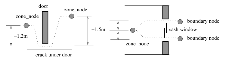
Nodes
In the left of the figure the two zone nodes are of type unknown pressure internal because we want to evaluate the pressure of the air in the zones. In the right of the figure there are two boundary nodes of type wind-driven boundary node. At simulation time the current wind speed and direction are converted into a pressure at the facade and used, along with the flow characteristics of the opening components to evaluate the flow. The node types available in ESP-r are:
Wind pressures
ESP-r includes a database of pressure coefficient sets. Each set has values at eight directions (22.5 degree intervals) which characterise the pressure relationship for a specific device. The user is tasked with supplying these values - perhaps from a wind-tunnel test or a CFD run.
Components
In the figure above a crack component (see below) was used to represent an undercut at a door. The shape of the undercut is not a good fit for a common orifice component. Simple air flow components (see below) were used to represent the top and bottom of the sash window. We could also have used a common orifice component.
Components which are based on curve fits:
Components that induce or restrict flow (e.g. ducts, valves) are typified by the following:
Components associated with architectural elements such as windows, cracks and doors are typified by:
Linkages
In the figure above flow paths are defined via the syntax of node X is connected to node Y via component Z where Z is D1 distance above/below X and Z is D2 distance above/below Y. The crack is below the two zone nodes and thus the D1 and D2 are negative. For the sash window, lets assume that the boundary nodes heights were set to be the centre of each opening. The D1 values are from the point of the height of the zone node and the D2 values will be zero.
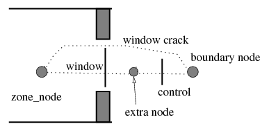
Control
In ESP-r, most flow components can have control imposed (but we would not impose control a crack). Control follows the general ESP-r pattern of defining the location of the sensor, what it senses, defining the component to be actuated as well as a schedule (for each day type) of control laws (control logic). For example control applied to an air flow opening or orifice would inpose a different area and control applied to a bi-directional component would alter the width of the opening.
Simple controls which act on a component can be associated with the following control actions:
Some control actions are more complex and one approach is to adjust the topology of the network so that controls can be placed in series as in the image below. Flow along the path is only possible when both the window control control and the additional component controller agree.
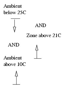
An alternative is to use a multi-sensor flow controlM/i> in which
multiple sensors and multiple AND OR logic states. It starts with a
default position (either open or closed) and changes (i.e. close or open) the
connection/component according to up to four logical AND/OR conditions
as in the figure below.
Relationship with other solvers
Discussion ... In XX the flow solution [preceeds/follows] the zone solution and ...
In XX the flow solution [preceeds/follows] the system solution and ...
A network flow solution supersedes scheduled air movement defintions. Users can bein with scheduled flows (imposed) and then create a flow network.
Back to top | Back to Welcome page