Methodology

Flow Duration Curve

The methodology which follows in this text is for the first two sites, Auchleshie and Keltie Bridge. For the third site there is a distinctive property which makes the area to differ from the first two sites and I will mention this later.
To measure the flow-rate of our sites, we first tried measuring the flow rate directly by throwing a floatable devise in the river. Then by measuring the time it took to travel over a set distance we could work out the flow-rate by using the distance equals speed over time calculation. However this had too many errors in this method, such as river turbulence, human error, friction and other properties of the floating device used. So we decided to abandon this for a more robust option.
The more robust option was to find out the flow-rate by working out the volume of water that was entering the river. So using the rainfall data which met office in UK provided us we tried to make a decent final hydro data for both cases. The difficulties we faced were a lot and some times were too complicated. Of course we were amateurs in such feasibility study and the first weeks were too difficult to us until we understood what we real should do.
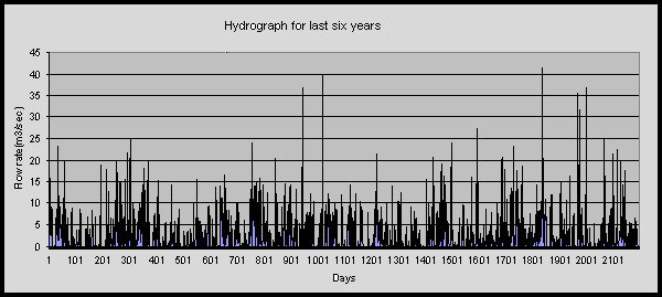
So the first step was to create the hydrograph for both sides. The most important step in a hydrograph is to calculate the flow rate of the river (direct flow). The flow rate can be calculated easily if you know the catchment area for your specific river and you have the appropriate rainfall data (monthly, daily or hourly). Catchment area is the area from which rain water flows into the specific river and we calculated it using the appropriate maps and ordinations for that area. Also provide us with these areas the institute of hydrology and we used this information in case to compare our results with the institute. So using the above equation you can calculate the flow rate:

Q = (AxR)/T

Where:
Q =Flow Rate (m3/sec)
A=Catchment Area (m2)
R = Annual Rainfall (m)
T= Time (sec)
In our case firstly we make a hydrograph using monthly rainfall data but because we didn’t have accuracy in our results we thought to use daily, as and it happened. So we use the rainfall data for a period of 6 years 2000-2006 and we calculated for this period of time the flow rate in both of our rivers (see excel sheet). Then we correlated the flow rate with time. This is done by putting in y axis flow rate values and in x axis the time in days So we took a descent hydrograph for both sites (see excel sheet).
The next step was to create the flow duration curve. This was the most crucial step for the entire project because with a good and accurate flow duration curve we should be able to choose the appropriate type of turbine for our sites. But to create a flow duration curve wasn’t as easy as we were thinking in the beginning. This because firstly we didn’t know how to make a flow duration curve and secondly we didn’t count something very important for a river, its base flows. After many days of searching and asking many hydrologists we managed to overcome with this complicated problem and we found a descent method to making flow duration curves and to calculate properly base flows.
So the first thing we did was to calculate base flow for both rivers and then add this flow to the direct flow (we mentioned before), this will now be known as total flow (see excel sheet). Now to calculate the base flow of a river wasn’t and the easiest thing. There are 3 different methods of calculating base flow in a river. We used the simplest one which also called “straight line method” (see excel sheet). In the beginning we made separately for each year the hydrographs. Hydrograph for last 6 years
From these 6 different hydrographs we chose the driest period which for each year was the same, between 1 of May and 30 of September. Then we delete zero days from the hydrograph and we use only the days with some rainfall. So now we had a number of different events for each year. Using these events and with the help of straight line method we managed to calculate the base flow for each of these events. At the end we took the average base flow of all these events and we found a final one which was the base flow for our river. We also should mention that we use just the driest period to calculate base flow for our rivers because if there is enough water those days, enough base flow, means that during the whole year there will be enough water inside the river, so never dry.
After we had calculated base flow we were ready to make the flow duration curve. The flow duration curve is a means of showing the probability in a graphical form of how many days in a year a particular flow will be exceeded. For example, it can be used to show the percentage of time river flow can be expected to exceed a design flow of some specified value (e.g., 20% of the time), or to show the discharge of the stream that occurs or is exceeded some percent of the time (e.g., 80% of the time). So using our total flow y axes and the percentage of time x axes we were be able to make flow duration curve for both sites. The technique to create a flow duration curve is quite simple and the steps are given below (see excel sheet):

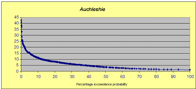
Step 1: Sort (rank) average daily discharges for period of record from the largest value to the smallest value, involving a total of n values.
Step 2: Assign each discharge value a rank (M), starting with 1 for the largest daily discharge value.
Step 3: Calculate exceedence probability (P) as follows:

P = 100 x [M / (n + 1)]

Where:
P = the probability that a given flow will be equalled or exceeded (% of time)
M = the ranked position on the listing (dimensionless)
n = the number of events for period of record (dimensionless)

Finally we were be able now with the help of course of the descent flow duration curve we made to continue in the other step which was to chose the appropriate type of turbine.

The straight line method

The straight line method is the simplest method to separate base flow. The base flow is separated by drawing a straight line joining the start and the end of direct runoff. The start of direct runoff (point A) can be determined by locating the point on the rising limb where there is a sharp increase in the runoff rate. The end of direct runoff (point B) can be easily determined by considering the last observation point on the data sheet provided. If point B is not well defined, draw a horizontal line from point A. These two points are then joined by a straight line. The area above this line is the direct runoff and the area below it is the base flow.

The intersection method

The intersection method is difference from the straight line method because it needs additional point in order to draw the separation line. This additional point is called the intersection point located at point C in Figure. Point C can be determined by extending the curve before point A until it intersects a vertical line drawn from the peak. Point C is then connected to point D on the recession curve. Point D can be determined by offsetting the time, N after the peak using the empirical equation:

N = 0.8 A02

Where N is the time after the peak in days and A is the catchments area in km2 The line AC and CD separate the flow into base flow and direct flow.

The recession curve method

In this method, the base flow recession curve is extrapolated backwards until it intersects the ordinate at the inflection point on the falling limb (point E). Point A and point E are then joined by an arbitrary curve. Lastly, point E is joined to point B on the recession curve as shown in the below Figure. The base flow is separated by considering the area under the lines AE and EB.
Here, the straight line method is simply called method 1, the intersection method is called method 2, and the recession curve method is called method 3 as shown in the above figure.

This figure shows flood hydrograph together with all the three separations methods use to separate the base flow.

Turbine Selection

The purpose of all turbines is to convert the energy from the falling water into the rotating shaft power. This is one of the most efficient way of getting energy from water. To select a turbine for a specific situation is a great challenge as it will directly affect the total power generate from that scheme.

Selection Criteria of Turbines

The selection of turbines depends upon following factors...

Site characteristics
Head of the hydro scheme
Flow rate available in the scheme
Desired runner speed of the generator
The probability of operating the turbine at reduced flow rates

Classification:
I ) Classification on the basis of head of water:
In these the turbines runner operate in air and driven by a jet of water These includes following turbines

High head
Medium head
Low head

For the generation of electricity from water, it is required that the there should me minimum difference from the speed of generator and turbine, so the shaft speed is required as close as possible to 1500rpm to minimize this difference in speeds. Also the speed of turbines declines with heads, so the low head schemes require faster turbines as compared with high head.

II )Classification on the basis of principle of operation:
a )Impulse Turbines
In these the turbines runner operate in air and driven by a jet of water
These includes following turbines:

Pelton
Turgo
Cross flow

b )Reaction Turbines:
The rotor of these turbines are fully immersed in water and enclosed in a pressure casing. The lift forces are produced by the pressure differences across the runner blades, similar as on aircraft wings, which cause the runner to rotate. These includes,

Propeller (with Kaplan variant)
Francis

Types of Turbines
1 ) Impulse Turbines Pelton turbines are composed of a wheel which carries a series of split buckets set around its rim; these buckets are strike tangentially with high velocity jet of water. In this way the falling water transfers all its energy to the buckets which then deflect at 180 degree.
Turgo turbines are similar to pelton but the water strikes at the plane of runner at an angle. So the water enters the runner at angle from one side and discharge from the other side. As it has no affect of the discharge being encountered with the incoming jet (as it was in pelton), the size of these machines will be smaller as compared with the pelton machine of same power output. Cross flow turbines consists of drum like rotor with a solid disk at each end and gutter shaped slats joining the two disks. In this operation of turbines, the jet of water enters at the top of rotor through blades and again emerged through the blades second times before discharged. These machines hoarsened maximum energy from the water as the waster transfer its momentum twice before leaving the system.
2 ) Reaction Turbines: All reaction turbines catch energy from the coming water by generating the hydrodynamic lift forces to propel the runner blades. The main difference between the impulse and reaction turbines is the runners of reaction turbines always functions within a completely water filled casing. The diffuser in the reaction turbines which is known as “draft tube” exist below the runner is for the discharge of water. It is also function to reduce the static pressure below the runner which ultimately causes to increase the effective head of scheme.
Propeller Type turbines are similar in principle to ship but operate in reversed mode. For higher efficiency water should be given a swirl before entering the turbine runner. For this guide vanes and snail shell housing is the practice to achieve the maximum efficiency of these turbines. Often these guide vanes are adjustable to permit the flow that enters into the turbine. In some designs the blades of the runner are also adjustable, so these are called Kaplan.
Francis turbine is modified form of propeller turbines. In these turbines the water flows radially inwards into the runner and turned to emerge axially. For medium head schemes runners are mounted in a spiral casing with internal adjustable guide vanes.

Head and Flow Ranges of Small Turbines

The Efficiency of Turbines:
The relative efficiencies of different turbines can be compared at

Design point
At reduced flow rate

Efficiencies comparison of different turbines at reduced flow rates

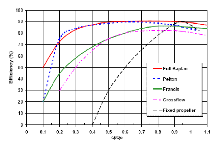
From the efficiencies comparison chart, it is evident that Pelton and Kaplan turbines retain their high efficiencies when running below design flow, but the efficiency of cross flow and Francis turbines falls sharply as they are operated below half of their design flow.
Reasons of Selecting Hydro-ekids for our Sites:
As it is evident from the Annual hydro graph and Flow Duration Curve, the sites have very low flow rate especially in summer and very high in the winter. So keeping in view of the site specifications and flow rate changing, we need a turbine which can work within a wide range of flow rates. So hydro-ekids which is propeller type turbines which can work within a wide range of flow rate.
The head of these sites comes under the range of these turbines.
Technically the cross flow and Francis turbines losses their efficiencies as the flow rate declines than the design flow of them, but propeller types turbines maintain their higher efficiency up to very low flow rate.
Because of higher efficiency the annual output of these turbines is much higher as compared with cross flow turbines which will leads to lower p/Kwh.
Higher costs of them are justified by their higher efficiency.
The design of these turbines is more compact
These require less construction costs as needed in the case of cross flow turbines
These require reduced volume of concrete for foundation as generator can be mounted on the turbine structure.
These can be used various site specifications.
Toshiba hydro-ekids type M:

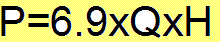
By using the above formula we could insert the results from the data such as Flow rate (Q) and Head (H). This would then gives us the expect power that would be produced by the turbine. The equation also takes account of all assumption such as frictional losses of the turbine at a rate of 70% very conservative. This leads the results to be on the safe side and therefore power would be expected to have an error of positive 1-3% but not anything less. After working out the power we can then use the three variables as criteria conditions for choosing the turbine. The way that we selected the turbine was to find as many turbines that fitted within those criteria conditions. Then we narrowed down the selection by choosing only those turbines that can either produce enough power to match the demand or be as close to it as possible. This gave us the short list we needed and then chose the Toshiba e-Kid M based on its competitive price and the design of the system.