CFD solvers
The CFD solver in ESP-r is in-built, and can be strongly coupled to other domains (see below). For more in-depth details the reader is referred to the various PhD theses detailing the development of CFD functionailty in ESP-r:
- Beausoleil-Morrison I (2000) 'The Adaptive Coupling of Heat and Air Flow Modelling Within Dynamic Whole-Building Simulation', PhD Thesis, Glasgow: University of Strathclyde.
- Negrao C O R (1995) 'Conflation of computational fluid dynamics and building thermal simulation', PhD Thesis, Glasgow: University of Strathclyde.
Furthermore, many of the formulations used in the method employed by ESP-r can be found in the following references:
- Versteeg H K and Malalasekera W (2007) 'An Introduction to Computational Fluid Dynamics: The Finite Volume Method' (2nd Edn). ISBN 9780131274983.
- Patankar S V (1980) 'Numerical Heat Transfer and Fluid Flow'. ISBN 9780891165224.
Numerical approach
ESP-r employs hybrid, fully implicit discretisation of finite volume CFD domains, and solves the resulting system of equations according to the SIMPLEC algorithm, using a convenient combination of TDMA and the Gauss-Seidel Iterative method.
Steady-state and transient assessments
The CFD in ESP-r is fully transient in both a technical and practical sense. Transient convection-diffusion equations are used, meaning the procedure is suitable for unsteady flows, and an assessment is (by default) performed for each building time-step, with dynamically updated boundary conditions (see below).
CFD sharing with other domains
CFD domains can be explicitly linked with the building and/or mass flow domains in ESP-r. The theoretical basis and computational implementation of these solvers are well documented in Clarke J A (2001) 'Energy Simulation in Building Design' (2nd Edn). ISBN 0750650826. Coupled domains exchange information with the CFD domain on a time-step basis, supplying the CFD with updated boundary conditions, and receiving local air flow and heat transfer data in return. The Adaptive Conflation Controller (ACC) developed by Beausoleil-Morrison (2000) gives some intelligence to this coupling process (see below).
The coupling with the mass flow domain in ESP-r is particularly noteworthy, as an iterative procedure is used to leverage the two solvers to achieve a mutual solution that effectively applies the global constraints of the inter-zonal mass flow network to all associated intra-zonal CFD domains. To the groups knowledge, no comparable coupling system is currently available in other programs.
CFD cells as sources
ESP-r has functionality to model solid boundaries, air flow openings at boundaries, heat and contaminant sources and sinks anywhere in the domain, and solid blockages (which may have an associated heat flux) anywhere in the domain. In most cases these local entities in the CFD domain can be linked to more nebulous entities in other domains, and therefore dynamically updated. For example a heat source could be associated with a casual gain in the building domain, or a contaminant source could be associated with a source in the contaminant network in the mass flow domain, etc.
CFD performance metrics
During simulations convergence information is recorded; by default scalar values at a specified monitoring cell and residuals are stored at appropriate intervals of iterations for each CFD assessment. If the ACC is used, salient information and resulting decisions are also stored. Users can retrieve output in graphical form (e.g. contour plots, flow field visualisations), or a variety of textual formats compatible with a range of commonly used 3rd party visualisation programs e.g. TECplot, ParaView.
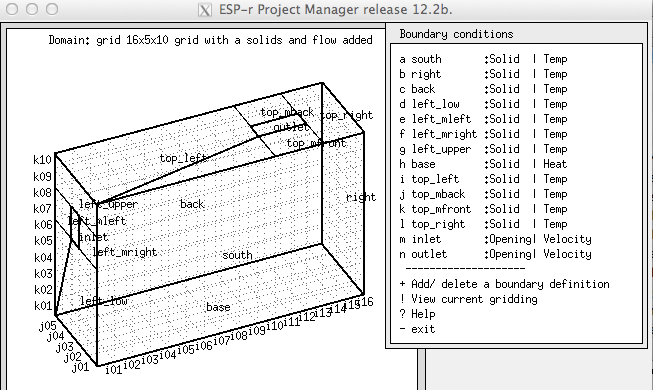
CFD domains
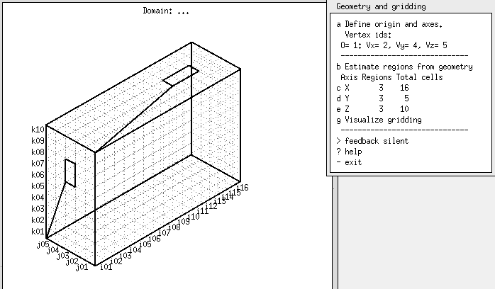
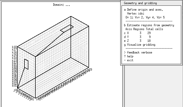
CFD domains in ESP-r are almost always rectilinear, and are constrained to hexahedral grid cells. Grid resolution is typically coarse in comparison to many other indoor air applications of CFD, due mainly to the lack of need for detailed "micro" air flow assessments in typical building simulation and the large computational burden that CFD places on the rest of the simulation. By default grid size is limited to 36 cells on each axis. In the figure below on the left is a low resolution (16 x 5 x 10) grid which solves quickly. On the right is the same space but with an even 100mm gridding.
Computational choices
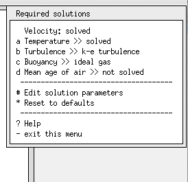
Turbulence can be modelled by a variety of techniques: 1) none (laminar flow), 2) fixed eddy viscosity, 3) de-facto standard k-epsilon model and 4) zero-equation algebraic model of Chen and Xu (1998). By default the ACC uses the k-eplison model, which allows it to most effectively tailor each simulation to prevailing flow conditions.
ESP-r contains a comprehensive set of built-in wall functions that include standard log-law and Yuan formulations. By default the ACC assesses general flow conditions at each time step, and hence choose the most appropriate wall functions for each assessment.
Buoyancy can be represented in the CFD equations using the Boussinesq approximation, full ideal gas law calculations, or not at all. By default the ACC assesses whether buoyancy is a significant driving factor, and therefore worth simulating, at each time step.
As well as standard scalar metrics (velocity, temperature, turbulence energy), ESP-r can also calculate, record and output local contaminant concentration and mean age of air during simulations.
Computational resources
CFD has a vastly greater computational requirement than any other simulation domain in ESP-r, so grid resolution is intentionally limited (see above). Generally speaking, on a reasonably up-to-date computer, one can expect very coarse CFD grids (~10 cells on each axis) to simulate in a matter of seconds per time step, and fine grids (50-100 cells on each axis) to simulate in the order of minutes per time step. The latter is supported if ESP-r has been compiled to support complex models. However it is important to point out that the computing resources required depend on a wide variety of factors, including the domain complexity in other respects, coupling to other domains, the time step, how quickly things change in the building, etc.
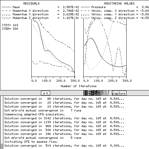
Views of slowly evolving convergence do not necessarly help us confirm that the design of the CFD domain has captured the performance of our design. And for assessments over several hundreds or thousands of timesteps the implications on workflows is considerable. The simulator includes an option to display the domain solution as the simulation progresses. An example is shown below:
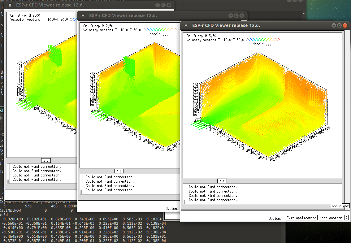 see full size
User controls
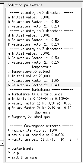
CFD convergence criteria in ESP-r must be specified as a maximum residual. If all velocity and mass residuals are below this threshold, the simulation is considered to have converged.
 see full size
Dependencies on the data model
Most CFD entities can be explicitly linked with entities in other domains, such as solid surfaces, air flow openings, heat and contaminant sources and sinks, etc. This creates an implicit association which then ensures the appropriate data structures are kept synchronised. Clearly in order to make physical sense, this requires that the geometry of the CFD domain is broadly similar to that of the building model. To this end, CFD domain geometry is first defined in terms of room vertices from the building side, and gridding can be inferred from room geometry algorithmically.
Back to top | Back to Welcome page